Jacobi's theta function θ 1 q = e i πτ e 0.1i π
θ
1
(
z
,
q
)
=
2
q
1
4
∑
n
=
0
∞
(
−
1
)
n
q
n
(
n
+
1
)
sin
(
2
n
+
1
)
z
=
∑
n
=
−
∞
∞
(
−
1
)
n
−
1
2
q
(
n
+
1
2
)
2
e
(
2
n
+
1
)
i
z
.
{\displaystyle {\begin{aligned}\theta _{1}(z,q)&=2q^{\frac {1}{4}}\sum _{n=0}^{\infty }(-1)^{n}q^{n(n+1)}\sin(2n+1)z\\&=\sum _{n=-\infty }^{\infty }(-1)^{n-{\frac {1}{2}}}q^{\left(n+{\frac {1}{2}}\right)^{2}}e^{(2n+1)iz}.\end{aligned}}}
In mathematics , theta functions are special functions of several complex variables . Fundamentally, they are a family of continuous functions which encode the behavior of discrete multi-dimensional periodic systems, such as crystal lattices or points on a torus . Because they are smooth, they allow the study and manipulation of discrete combinatorial systems using the tools of analysis .
For this reason, theta functions have useful applications in topics such as
number theory : "in how many ways can a number be written as a sum of squares?"physics : "how does heat flow on a toroidal ring?", "how do quantum particles behave when arranged in a lattice?"geometry : "what are the shape properties of elliptic curves ?"and others, including abelian varieties , moduli spaces , quadratic forms , and solitons .
Theta functions in two dimensions are functions of two complex arguments. In one choice of parameter, for example,
z
{\displaystyle z}
τ
{\displaystyle \tau }
q
{\displaystyle q}
tube domain inside a complex Lagrangian Grassmannian ,[ 1] Siegel upper half space .
Basic example
edit
One example of a theta function is
θ
(
z
,
q
)
≡
∑
n
=
−
∞
∞
q
n
2
exp
(
2
π
i
n
z
)
{\displaystyle \theta (z,q)\equiv \sum _{n=-\infty }^{\infty }q^{n^{2}}\exp {(2\pi inz)}}
where
z
{\displaystyle z}
q
{\displaystyle q}
|
q
|
<
1
{\displaystyle |q|<1}
This analytic function can be used to solve a combinatorics problem: in how many different ways can an integer be written as the sum of two squares? When
z
=
0
{\displaystyle z=0}
θ
(
0
,
q
)
=
∑
n
=
−
∞
∞
q
n
2
=
1
+
2
q
+
2
q
4
+
2
q
9
+
…
+
2
q
n
2
+
…
{\displaystyle \theta (0,q)=\sum _{n=-\infty }^{\infty }q^{n^{2}}=1+2q+2q^{4}+2q^{9}+\ldots +2q^{n^{2}}+\ldots }
This is a generating function where the coefficient of
q
k
{\displaystyle q^{k}}
k
{\displaystyle k}
k
=
0
{\displaystyle k=0}
k
{\displaystyle k}
n
2
=
(
−
n
)
2
{\displaystyle n^{2}=(-n)^{2}}
k
{\displaystyle k}
Squaring this generating function, we obtain
θ
(
0
,
q
)
2
=
(
∑
m
q
m
2
)
(
∑
n
q
n
2
)
=
∑
m
,
n
q
m
2
+
n
2
{\displaystyle \theta (0,q)^{2}={\Bigl (}\sum _{m}q^{m^{2}}{\Bigr )}{\Bigl (}\sum _{n}q^{n^{2}}{\Bigr )}=\sum _{m,n}q^{m^{2}+n^{2}}}
Collecting terms by exponent, we find that
θ
(
0
,
q
)
2
{\displaystyle \theta (0,q)^{2}}
q
k
{\displaystyle q^{k}}
k
{\displaystyle k}
(
3
,
4
)
{\displaystyle (3,4)}
(
4
,
3
)
{\displaystyle (4,3)}
(
−
3
,
4
)
{\displaystyle (-3,4)}
3
2
+
4
2
=
25
{\displaystyle 3^{2}+4^{2}=25}
Application to elliptic functions
edit
Theta functions occur most commonly in the theory of elliptic functions . With respect to one of the complex variables
z
{\displaystyle z}
quasiperiodic function . Abstractly, this quasiperiodicity comes from the cohomology class of a line bundle on a complex torus , a condition of descent .
One interpretation of theta functions when dealing with the heat equation is that "a theta function is a special function that describes the evolution of temperature on a segment domain subject to certain boundary conditions".[ 2]
Throughout this article,
(
e
π
i
τ
)
α
{\displaystyle (e^{\pi i\tau })^{\alpha }}
e
α
π
i
τ
{\displaystyle e^{\alpha \pi i\tau }}
branch ).[ note 1]
Jacobi theta function
edit
There are several closely related functions called Jacobi theta functions, and many different and incompatible systems of notation for them.
One Jacobi theta function (named after Carl Gustav Jacob Jacobi ) is a function defined for two complex variables z and τ , where z can be any complex number and τ is the half-period ratio , confined to the upper half-plane , which means it has a positive imaginary part. It is given by the formula
ϑ
(
z
;
τ
)
=
∑
n
=
−
∞
∞
exp
(
π
i
n
2
τ
+
2
π
i
n
z
)
=
1
+
2
∑
n
=
1
∞
q
n
2
cos
(
2
π
n
z
)
=
∑
n
=
−
∞
∞
q
n
2
η
n
{\displaystyle {\begin{aligned}\vartheta (z;\tau )&=\sum _{n=-\infty }^{\infty }\exp \left(\pi in^{2}\tau +2\pi inz\right)\\&=1+2\sum _{n=1}^{\infty }q^{n^{2}}\cos(2\pi nz)\\&=\sum _{n=-\infty }^{\infty }q^{n^{2}}\eta ^{n}\end{aligned}}}
where q = exp(πiτ )nome and η = exp(2πiz )Jacobi form . The restriction ensures that it is an absolutely convergent series. At fixed τ , this is a Fourier series for a 1-periodic entire function of z . Accordingly, the theta function is 1-periodic in z :
ϑ
(
z
+
1
;
τ
)
=
ϑ
(
z
;
τ
)
.
{\displaystyle \vartheta (z+1;\tau )=\vartheta (z;\tau ).}
By completing the square , it is also τ -quasiperiodic in z , with
ϑ
(
z
+
τ
;
τ
)
=
exp
(
−
π
i
(
τ
+
2
z
)
)
ϑ
(
z
;
τ
)
.
{\displaystyle \vartheta (z+\tau ;\tau )=\exp {\bigl (}-\pi i(\tau +2z){\bigr )}\vartheta (z;\tau ).}
Thus, in general,
ϑ
(
z
+
a
+
b
τ
;
τ
)
=
exp
(
−
π
i
b
2
τ
−
2
π
i
b
z
)
ϑ
(
z
;
τ
)
{\displaystyle \vartheta (z+a+b\tau ;\tau )=\exp \left(-\pi ib^{2}\tau -2\pi ibz\right)\vartheta (z;\tau )}
for any integers a and b .
For any fixed
τ
{\displaystyle \tau }
Liouville's theorem , it cannot be doubly periodic in
1
,
τ
{\displaystyle 1,\tau }
1
{\displaystyle 1}
τ
{\displaystyle \tau }
|
ϑ
(
z
+
a
+
b
τ
;
τ
)
ϑ
(
z
;
τ
)
|
=
exp
(
π
(
b
2
ℑ
(
τ
)
+
2
b
ℑ
(
z
)
)
)
{\displaystyle \left|{\frac {\vartheta (z+a+b\tau ;\tau )}{\vartheta (z;\tau )}}\right|=\exp \left(\pi (b^{2}\Im (\tau )+2b\Im (z))\right)}
ℑ
(
τ
)
>
0
{\displaystyle \Im (\tau )>0}
ϑ
(
z
,
τ
)
{\displaystyle \vartheta (z,\tau )}
It is in fact the most general entire function with 2 quasi-periods, in the following sense:[ 3]
Theta function θ 1 q = e iπτ q changes with τ . Theta function θ 1 q = e iπτ q changes with τ .
Auxiliary functions
edit
The Jacobi theta function defined above is sometimes considered along with three auxiliary theta functions, in which case it is written with a double 0 subscript:
ϑ
00
(
z
;
τ
)
=
ϑ
(
z
;
τ
)
{\displaystyle \vartheta _{00}(z;\tau )=\vartheta (z;\tau )}
The auxiliary (or half-period) functions are defined by
ϑ
01
(
z
;
τ
)
=
ϑ
(
z
+
1
2
;
τ
)
ϑ
10
(
z
;
τ
)
=
exp
(
1
4
π
i
τ
+
π
i
z
)
ϑ
(
z
+
1
2
τ
;
τ
)
ϑ
11
(
z
;
τ
)
=
exp
(
1
4
π
i
τ
+
π
i
(
z
+
1
2
)
)
ϑ
(
z
+
1
2
τ
+
1
2
;
τ
)
.
{\displaystyle {\begin{aligned}\vartheta _{01}(z;\tau )&=\vartheta \left(z+{\tfrac {1}{2}};\tau \right)\\[3pt]\vartheta _{10}(z;\tau )&=\exp \left({\tfrac {1}{4}}\pi i\tau +\pi iz\right)\vartheta \left(z+{\tfrac {1}{2}}\tau ;\tau \right)\\[3pt]\vartheta _{11}(z;\tau )&=\exp \left({\tfrac {1}{4}}\pi i\tau +\pi i\left(z+{\tfrac {1}{2}}\right)\right)\vartheta \left(z+{\tfrac {1}{2}}\tau +{\tfrac {1}{2}};\tau \right).\end{aligned}}}
This notation follows Riemann and Mumford ; Jacobi 's original formulation was in terms of the nome q = e iπτ τ . In Jacobi's notation the θ -functions are written:
θ
1
(
z
;
q
)
=
θ
1
(
π
z
,
q
)
=
−
ϑ
11
(
z
;
τ
)
θ
2
(
z
;
q
)
=
θ
2
(
π
z
,
q
)
=
ϑ
10
(
z
;
τ
)
θ
3
(
z
;
q
)
=
θ
3
(
π
z
,
q
)
=
ϑ
00
(
z
;
τ
)
θ
4
(
z
;
q
)
=
θ
4
(
π
z
,
q
)
=
ϑ
01
(
z
;
τ
)
{\displaystyle {\begin{aligned}\theta _{1}(z;q)&=\theta _{1}(\pi z,q)=-\vartheta _{11}(z;\tau )\\\theta _{2}(z;q)&=\theta _{2}(\pi z,q)=\vartheta _{10}(z;\tau )\\\theta _{3}(z;q)&=\theta _{3}(\pi z,q)=\vartheta _{00}(z;\tau )\\\theta _{4}(z;q)&=\theta _{4}(\pi z,q)=\vartheta _{01}(z;\tau )\end{aligned}}}
Jacobi theta 1 Jacobi theta 2 Jacobi theta 3 Jacobi theta 4 The above definitions of the Jacobi theta functions are by no means unique. See Jacobi theta functions (notational variations) for further discussion.
If we set z = 0τ only, defined on the upper half-plane. These functions are called Theta Nullwert functions, based on the German term for zero value because of the annullation of the left entry in the theta function expression. Alternatively, we obtain four functions of q only, defined on the unit disk
|
q
|
<
1
{\displaystyle |q|<1}
theta constants :[ note 2]
ϑ
11
(
0
;
τ
)
=
−
θ
1
(
q
)
=
−
∑
n
=
−
∞
∞
(
−
1
)
n
−
1
/
2
q
(
n
+
1
/
2
)
2
ϑ
10
(
0
;
τ
)
=
θ
2
(
q
)
=
∑
n
=
−
∞
∞
q
(
n
+
1
/
2
)
2
ϑ
00
(
0
;
τ
)
=
θ
3
(
q
)
=
∑
n
=
−
∞
∞
q
n
2
ϑ
01
(
0
;
τ
)
=
θ
4
(
q
)
=
∑
n
=
−
∞
∞
(
−
1
)
n
q
n
2
{\displaystyle {\begin{aligned}\vartheta _{11}(0;\tau )&=-\theta _{1}(q)=-\sum _{n=-\infty }^{\infty }(-1)^{n-1/2}q^{(n+1/2)^{2}}\\\vartheta _{10}(0;\tau )&=\theta _{2}(q)=\sum _{n=-\infty }^{\infty }q^{(n+1/2)^{2}}\\\vartheta _{00}(0;\tau )&=\theta _{3}(q)=\sum _{n=-\infty }^{\infty }q^{n^{2}}\\\vartheta _{01}(0;\tau )&=\theta _{4}(q)=\sum _{n=-\infty }^{\infty }(-1)^{n}q^{n^{2}}\end{aligned}}}
with the nome q = e iπτ
θ
1
(
q
)
=
0
{\displaystyle \theta _{1}(q)=0}
modular forms , and to parametrize certain curves; in particular, the Jacobi identity is
θ
2
(
q
)
4
+
θ
4
(
q
)
4
=
θ
3
(
q
)
4
{\displaystyle \theta _{2}(q)^{4}+\theta _{4}(q)^{4}=\theta _{3}(q)^{4}}
or equivalently,
ϑ
01
(
0
;
τ
)
4
+
ϑ
10
(
0
;
τ
)
4
=
ϑ
00
(
0
;
τ
)
4
{\displaystyle \vartheta _{01}(0;\tau )^{4}+\vartheta _{10}(0;\tau )^{4}=\vartheta _{00}(0;\tau )^{4}}
which is the Fermat curve of degree four.
Jacobi identities
edit
Jacobi's identities describe how theta functions transform under the modular group , which is generated by τ ↦ τ + 1τ ↦ −1 / τ τ in the exponent has the same effect as adding 1 / 2 to z (n ≡ n 2 mod 2
α
=
(
−
i
τ
)
1
2
exp
(
π
τ
i
z
2
)
.
{\displaystyle \alpha =(-i\tau )^{\frac {1}{2}}\exp \left({\frac {\pi }{\tau }}iz^{2}\right).}
Then
ϑ
00
(
z
τ
;
−
1
τ
)
=
α
ϑ
00
(
z
;
τ
)
ϑ
01
(
z
τ
;
−
1
τ
)
=
α
ϑ
10
(
z
;
τ
)
ϑ
10
(
z
τ
;
−
1
τ
)
=
α
ϑ
01
(
z
;
τ
)
ϑ
11
(
z
τ
;
−
1
τ
)
=
−
i
α
ϑ
11
(
z
;
τ
)
.
{\displaystyle {\begin{aligned}\vartheta _{00}\!\left({\frac {z}{\tau }};{\frac {-1}{\tau }}\right)&=\alpha \,\vartheta _{00}(z;\tau )\quad &\vartheta _{01}\!\left({\frac {z}{\tau }};{\frac {-1}{\tau }}\right)&=\alpha \,\vartheta _{10}(z;\tau )\\[3pt]\vartheta _{10}\!\left({\frac {z}{\tau }};{\frac {-1}{\tau }}\right)&=\alpha \,\vartheta _{01}(z;\tau )\quad &\vartheta _{11}\!\left({\frac {z}{\tau }};{\frac {-1}{\tau }}\right)&=-i\alpha \,\vartheta _{11}(z;\tau ).\end{aligned}}}
Theta functions in terms of the nome
edit
Instead of expressing the Theta functions in terms of z and τ , we may express them in terms of arguments w and the nome q , where w = e πiz q = e πiτ
ϑ
00
(
w
,
q
)
=
∑
n
=
−
∞
∞
(
w
2
)
n
q
n
2
ϑ
01
(
w
,
q
)
=
∑
n
=
−
∞
∞
(
−
1
)
n
(
w
2
)
n
q
n
2
ϑ
10
(
w
,
q
)
=
∑
n
=
−
∞
∞
(
w
2
)
n
+
1
2
q
(
n
+
1
2
)
2
ϑ
11
(
w
,
q
)
=
i
∑
n
=
−
∞
∞
(
−
1
)
n
(
w
2
)
n
+
1
2
q
(
n
+
1
2
)
2
.
{\displaystyle {\begin{aligned}\vartheta _{00}(w,q)&=\sum _{n=-\infty }^{\infty }\left(w^{2}\right)^{n}q^{n^{2}}\quad &\vartheta _{01}(w,q)&=\sum _{n=-\infty }^{\infty }(-1)^{n}\left(w^{2}\right)^{n}q^{n^{2}}\\[3pt]\vartheta _{10}(w,q)&=\sum _{n=-\infty }^{\infty }\left(w^{2}\right)^{n+{\frac {1}{2}}}q^{\left(n+{\frac {1}{2}}\right)^{2}}\quad &\vartheta _{11}(w,q)&=i\sum _{n=-\infty }^{\infty }(-1)^{n}\left(w^{2}\right)^{n+{\frac {1}{2}}}q^{\left(n+{\frac {1}{2}}\right)^{2}}.\end{aligned}}}
We see that the theta functions can also be defined in terms of w and q , without a direct reference to the exponential function. These formulas can, therefore, be used to define the Theta functions over other fields where the exponential function might not be everywhere defined, such as fields of p -adic numbers
Product representations
edit
The Jacobi triple product (a special case of the Macdonald identities ) tells us that for complex numbers w and q with |q and w ≠ 0
∏
m
=
1
∞
(
1
−
q
2
m
)
(
1
+
w
2
q
2
m
−
1
)
(
1
+
w
−
2
q
2
m
−
1
)
=
∑
n
=
−
∞
∞
w
2
n
q
n
2
.
{\displaystyle \prod _{m=1}^{\infty }\left(1-q^{2m}\right)\left(1+w^{2}q^{2m-1}\right)\left(1+w^{-2}q^{2m-1}\right)=\sum _{n=-\infty }^{\infty }w^{2n}q^{n^{2}}.}
It can be proven by elementary means, as for instance in Hardy and Wright's An Introduction to the Theory of Numbers
If we express the theta function in terms of the nome q = e πiτ q = e 2πiτ w = e πiz
ϑ
(
z
;
τ
)
=
∑
n
=
−
∞
∞
exp
(
π
i
τ
n
2
)
exp
(
2
π
i
z
n
)
=
∑
n
=
−
∞
∞
w
2
n
q
n
2
.
{\displaystyle \vartheta (z;\tau )=\sum _{n=-\infty }^{\infty }\exp(\pi i\tau n^{2})\exp(2\pi izn)=\sum _{n=-\infty }^{\infty }w^{2n}q^{n^{2}}.}
We therefore obtain a product formula for the theta function in the form
ϑ
(
z
;
τ
)
=
∏
m
=
1
∞
(
1
−
exp
(
2
m
π
i
τ
)
)
(
1
+
exp
(
(
2
m
−
1
)
π
i
τ
+
2
π
i
z
)
)
(
1
+
exp
(
(
2
m
−
1
)
π
i
τ
−
2
π
i
z
)
)
.
{\displaystyle \vartheta (z;\tau )=\prod _{m=1}^{\infty }{\big (}1-\exp(2m\pi i\tau ){\big )}{\Big (}1+\exp {\big (}(2m-1)\pi i\tau +2\pi iz{\big )}{\Big )}{\Big (}1+\exp {\big (}(2m-1)\pi i\tau -2\pi iz{\big )}{\Big )}.}
In terms of w and q :
ϑ
(
z
;
τ
)
=
∏
m
=
1
∞
(
1
−
q
2
m
)
(
1
+
q
2
m
−
1
w
2
)
(
1
+
q
2
m
−
1
w
2
)
=
(
q
2
;
q
2
)
∞
(
−
w
2
q
;
q
2
)
∞
(
−
q
w
2
;
q
2
)
∞
=
(
q
2
;
q
2
)
∞
θ
(
−
w
2
q
;
q
2
)
{\displaystyle {\begin{aligned}\vartheta (z;\tau )&=\prod _{m=1}^{\infty }\left(1-q^{2m}\right)\left(1+q^{2m-1}w^{2}\right)\left(1+{\frac {q^{2m-1}}{w^{2}}}\right)\\&=\left(q^{2};q^{2}\right)_{\infty }\,\left(-w^{2}q;q^{2}\right)_{\infty }\,\left(-{\frac {q}{w^{2}}};q^{2}\right)_{\infty }\\&=\left(q^{2};q^{2}\right)_{\infty }\,\theta \left(-w^{2}q;q^{2}\right)\end{aligned}}}
where ( ; )∞ is the q -Pochhammer symbolθ ( ; )q -theta function
∏
m
=
1
∞
(
1
−
q
2
m
)
(
1
+
(
w
2
+
w
−
2
)
q
2
m
−
1
+
q
4
m
−
2
)
,
{\displaystyle \prod _{m=1}^{\infty }\left(1-q^{2m}\right){\Big (}1+\left(w^{2}+w^{-2}\right)q^{2m-1}+q^{4m-2}{\Big )},}
which we may also write as
ϑ
(
z
∣
q
)
=
∏
m
=
1
∞
(
1
−
q
2
m
)
(
1
+
2
cos
(
2
π
z
)
q
2
m
−
1
+
q
4
m
−
2
)
.
{\displaystyle \vartheta (z\mid q)=\prod _{m=1}^{\infty }\left(1-q^{2m}\right)\left(1+2\cos(2\pi z)q^{2m-1}+q^{4m-2}\right).}
This form is valid in general but clearly is of particular interest when z is real. Similar product formulas for the auxiliary theta functions are
ϑ
01
(
z
∣
q
)
=
∏
m
=
1
∞
(
1
−
q
2
m
)
(
1
−
2
cos
(
2
π
z
)
q
2
m
−
1
+
q
4
m
−
2
)
,
ϑ
10
(
z
∣
q
)
=
2
q
1
4
cos
(
π
z
)
∏
m
=
1
∞
(
1
−
q
2
m
)
(
1
+
2
cos
(
2
π
z
)
q
2
m
+
q
4
m
)
,
ϑ
11
(
z
∣
q
)
=
−
2
q
1
4
sin
(
π
z
)
∏
m
=
1
∞
(
1
−
q
2
m
)
(
1
−
2
cos
(
2
π
z
)
q
2
m
+
q
4
m
)
.
{\displaystyle {\begin{aligned}\vartheta _{01}(z\mid q)&=\prod _{m=1}^{\infty }\left(1-q^{2m}\right)\left(1-2\cos(2\pi z)q^{2m-1}+q^{4m-2}\right),\\[3pt]\vartheta _{10}(z\mid q)&=2q^{\frac {1}{4}}\cos(\pi z)\prod _{m=1}^{\infty }\left(1-q^{2m}\right)\left(1+2\cos(2\pi z)q^{2m}+q^{4m}\right),\\[3pt]\vartheta _{11}(z\mid q)&=-2q^{\frac {1}{4}}\sin(\pi z)\prod _{m=1}^{\infty }\left(1-q^{2m}\right)\left(1-2\cos(2\pi z)q^{2m}+q^{4m}\right).\end{aligned}}}
In particular,
lim
q
→
0
ϑ
10
(
z
∣
q
)
2
q
1
4
=
cos
(
π
z
)
,
lim
q
→
0
−
ϑ
11
(
z
∣
q
)
2
q
1
4
=
sin
(
π
z
)
{\displaystyle \lim _{q\to 0}{\frac {\vartheta _{10}(z\mid q)}{2q^{\frac {1}{4}}}}=\cos(\pi z),\quad \lim _{q\to 0}{\frac {-\vartheta _{11}(z\mid q)}{2q^{\frac {1}{4}}}}=\sin(\pi z)}
sin
,
cos
{\displaystyle \sin ,\cos }
Integral representations
edit
The Jacobi theta functions have the following integral representations:
ϑ
00
(
z
;
τ
)
=
−
i
∫
i
−
∞
i
+
∞
e
i
π
τ
u
2
cos
(
2
π
u
z
+
π
u
)
sin
(
π
u
)
d
u
;
ϑ
01
(
z
;
τ
)
=
−
i
∫
i
−
∞
i
+
∞
e
i
π
τ
u
2
cos
(
2
π
u
z
)
sin
(
π
u
)
d
u
;
ϑ
10
(
z
;
τ
)
=
−
i
e
i
π
z
+
1
4
i
π
τ
∫
i
−
∞
i
+
∞
e
i
π
τ
u
2
cos
(
2
π
u
z
+
π
u
+
π
τ
u
)
sin
(
π
u
)
d
u
;
ϑ
11
(
z
;
τ
)
=
e
i
π
z
+
1
4
i
π
τ
∫
i
−
∞
i
+
∞
e
i
π
τ
u
2
cos
(
2
π
u
z
+
π
τ
u
)
sin
(
π
u
)
d
u
.
{\displaystyle {\begin{aligned}\vartheta _{00}(z;\tau )&=-i\int _{i-\infty }^{i+\infty }e^{i\pi \tau u^{2}}{\frac {\cos(2\pi uz+\pi u)}{\sin(\pi u)}}\mathrm {d} u;\\[6pt]\vartheta _{01}(z;\tau )&=-i\int _{i-\infty }^{i+\infty }e^{i\pi \tau u^{2}}{\frac {\cos(2\pi uz)}{\sin(\pi u)}}\mathrm {d} u;\\[6pt]\vartheta _{10}(z;\tau )&=-ie^{i\pi z+{\frac {1}{4}}i\pi \tau }\int _{i-\infty }^{i+\infty }e^{i\pi \tau u^{2}}{\frac {\cos(2\pi uz+\pi u+\pi \tau u)}{\sin(\pi u)}}\mathrm {d} u;\\[6pt]\vartheta _{11}(z;\tau )&=e^{i\pi z+{\frac {1}{4}}i\pi \tau }\int _{i-\infty }^{i+\infty }e^{i\pi \tau u^{2}}{\frac {\cos(2\pi uz+\pi \tau u)}{\sin(\pi u)}}\mathrm {d} u.\end{aligned}}}
The Theta Nullwert function
θ
3
(
q
)
{\displaystyle \theta _{3}(q)}
θ
3
(
q
)
=
1
+
4
q
ln
(
1
/
q
)
π
∫
0
∞
exp
[
−
ln
(
1
/
q
)
x
2
]
{
1
−
q
2
cos
[
2
ln
(
1
/
q
)
x
]
}
1
−
2
q
2
cos
[
2
ln
(
1
/
q
)
x
]
+
q
4
d
x
{\displaystyle \theta _{3}(q)=1+{\frac {4q{\sqrt {\ln(1/q)}}}{\sqrt {\pi }}}\int _{0}^{\infty }{\frac {\exp[-\ln(1/q)\,x^{2}]\{1-q^{2}\cos[2\ln(1/q)\,x]\}}{1-2q^{2}\cos[2\ln(1/q)\,x]+q^{4}}}\,\mathrm {d} x}
This formula was discussed in the essay Square series generating function transformations by the mathematician Maxie Schmidt from Georgia in Atlanta.
Based on this formula following three eminent examples are given:
[
2
π
K
(
1
2
2
)
]
1
/
2
=
θ
3
[
exp
(
−
π
)
]
=
1
+
4
exp
(
−
π
)
∫
0
∞
exp
(
−
π
x
2
)
[
1
−
exp
(
−
2
π
)
cos
(
2
π
x
)
]
1
−
2
exp
(
−
2
π
)
cos
(
2
π
x
)
+
exp
(
−
4
π
)
d
x
{\displaystyle {\biggl [}{\frac {2}{\pi }}K{\bigl (}{\frac {1}{2}}{\sqrt {2}}{\bigr )}{\biggr ]}^{1/2}=\theta _{3}{\bigl [}\exp(-\pi ){\bigr ]}=1+4\exp(-\pi )\int _{0}^{\infty }{\frac {\exp(-\pi x^{2})[1-\exp(-2\pi )\cos(2\pi x)]}{1-2\exp(-2\pi )\cos(2\pi x)+\exp(-4\pi )}}\,\mathrm {d} x}
[
2
π
K
(
2
−
1
)
]
1
/
2
=
θ
3
[
exp
(
−
2
π
)
]
=
1
+
4
2
4
exp
(
−
2
π
)
∫
0
∞
exp
(
−
2
π
x
2
)
[
1
−
exp
(
−
2
2
π
)
cos
(
2
2
π
x
)
]
1
−
2
exp
(
−
2
2
π
)
cos
(
2
2
π
x
)
+
exp
(
−
4
2
π
)
d
x
{\displaystyle {\biggl [}{\frac {2}{\pi }}K({\sqrt {2}}-1){\biggr ]}^{1/2}=\theta _{3}{\bigl [}\exp(-{\sqrt {2}}\,\pi ){\bigr ]}=1+4\,{\sqrt[{4}]{2}}\exp(-{\sqrt {2}}\,\pi )\int _{0}^{\infty }{\frac {\exp(-{\sqrt {2}}\,\pi x^{2})[1-\exp(-2{\sqrt {2}}\,\pi )\cos(2{\sqrt {2}}\,\pi x)]}{1-2\exp(-2{\sqrt {2}}\,\pi )\cos(2{\sqrt {2}}\,\pi x)+\exp(-4{\sqrt {2}}\,\pi )}}\,\mathrm {d} x}
{
2
π
K
[
sin
(
π
12
)
]
}
1
/
2
=
θ
3
[
exp
(
−
3
π
)
]
=
1
+
4
3
4
exp
(
−
3
π
)
∫
0
∞
exp
(
−
3
π
x
2
)
[
1
−
exp
(
−
2
3
π
)
cos
(
2
3
π
x
)
]
1
−
2
exp
(
−
2
3
π
)
cos
(
2
3
π
x
)
+
exp
(
−
4
3
π
)
d
x
{\displaystyle {\biggl \{}{\frac {2}{\pi }}K{\bigl [}\sin {\bigl (}{\frac {\pi }{12}}{\bigr )}{\bigr ]}{\biggr \}}^{1/2}=\theta _{3}{\bigl [}\exp(-{\sqrt {3}}\,\pi ){\bigr ]}=1+4\,{\sqrt[{4}]{3}}\exp(-{\sqrt {3}}\,\pi )\int _{0}^{\infty }{\frac {\exp(-{\sqrt {3}}\,\pi x^{2})[1-\exp(-2{\sqrt {3}}\,\pi )\cos(2{\sqrt {3}}\,\pi x)]}{1-2\exp(-2{\sqrt {3}}\,\pi )\cos(2{\sqrt {3}}\,\pi x)+\exp(-4{\sqrt {3}}\,\pi )}}\,\mathrm {d} x}
Furthermore, the theta examples
θ
3
(
1
2
)
{\displaystyle \theta _{3}({\tfrac {1}{2}})}
θ
3
(
1
3
)
{\displaystyle \theta _{3}({\tfrac {1}{3}})}
θ
3
(
1
2
)
=
1
+
2
∑
n
=
1
∞
1
2
n
2
=
1
+
2
π
−
1
/
2
ln
(
2
)
∫
0
∞
exp
[
−
ln
(
2
)
x
2
]
{
16
−
4
cos
[
2
ln
(
2
)
x
]
}
17
−
8
cos
[
2
ln
(
2
)
x
]
d
x
{\displaystyle \theta _{3}\left({\frac {1}{2}}\right)=1+2\sum _{n=1}^{\infty }{\frac {1}{2^{n^{2}}}}=1+2\pi ^{-1/2}{\sqrt {\ln(2)}}\int _{0}^{\infty }{\frac {\exp[-\ln(2)\,x^{2}]\{16-4\cos[2\ln(2)\,x]\}}{17-8\cos[2\ln(2)\,x]}}\,\mathrm {d} x}
θ
3
(
1
2
)
=
2.128936827211877158669
…
{\displaystyle \theta _{3}\left({\frac {1}{2}}\right)=2.128936827211877158669\ldots }
θ
3
(
1
3
)
=
1
+
2
∑
n
=
1
∞
1
3
n
2
=
1
+
4
3
π
−
1
/
2
ln
(
3
)
∫
0
∞
exp
[
−
ln
(
3
)
x
2
]
{
81
−
9
cos
[
2
ln
(
3
)
x
]
}
82
−
18
cos
[
2
ln
(
3
)
x
]
d
x
{\displaystyle \theta _{3}\left({\frac {1}{3}}\right)=1+2\sum _{n=1}^{\infty }{\frac {1}{3^{n^{2}}}}=1+{\frac {4}{3}}\pi ^{-1/2}{\sqrt {\ln(3)}}\int _{0}^{\infty }{\frac {\exp[-\ln(3)\,x^{2}]\{81-9\cos[2\ln(3)\,x]\}}{82-18\cos[2\ln(3)\,x]}}\,\mathrm {d} x}
θ
3
(
1
3
)
=
1.691459681681715341348
…
{\displaystyle \theta _{3}\left({\frac {1}{3}}\right)=1.691459681681715341348\ldots }
Explicit values
edit
Proper credit for most of these results goes to Ramanujan. See Ramanujan's lost notebook and a relevant reference at Euler function . The Ramanujan results quoted at Euler function plus a few elementary operations give the results below, so they are either in Ramanujan's lost notebook or follow immediately from it. See also Yi (2004).[ 4]
φ
(
q
)
=
ϑ
00
(
0
;
τ
)
=
θ
3
(
0
;
q
)
=
∑
n
=
−
∞
∞
q
n
2
{\displaystyle \quad \varphi (q)=\vartheta _{00}(0;\tau )=\theta _{3}(0;q)=\sum _{n=-\infty }^{\infty }q^{n^{2}}}
with the nome
q
=
e
π
i
τ
,
{\displaystyle q=e^{\pi i\tau },}
τ
=
n
−
1
,
{\displaystyle \tau =n{\sqrt {-1}},}
Dedekind eta function
η
(
τ
)
.
{\displaystyle \eta (\tau ).}
n
=
1
,
2
,
3
,
…
{\displaystyle n=1,2,3,\dots }
φ
(
e
−
π
)
=
π
4
Γ
(
3
4
)
=
2
η
(
−
1
)
φ
(
e
−
2
π
)
=
π
4
Γ
(
3
4
)
2
+
2
2
φ
(
e
−
3
π
)
=
π
4
Γ
(
3
4
)
1
+
3
108
8
φ
(
e
−
4
π
)
=
π
4
Γ
(
3
4
)
2
+
8
4
4
φ
(
e
−
5
π
)
=
π
4
Γ
(
3
4
)
2
+
5
5
φ
(
e
−
6
π
)
=
π
4
Γ
(
3
4
)
1
4
+
3
4
+
4
4
+
9
4
12
3
8
φ
(
e
−
7
π
)
=
π
4
Γ
(
3
4
)
13
+
7
+
7
+
3
7
14
3
8
⋅
7
16
φ
(
e
−
8
π
)
=
π
4
Γ
(
3
4
)
2
+
2
+
128
8
4
φ
(
e
−
9
π
)
=
π
4
Γ
(
3
4
)
1
+
2
+
2
3
3
3
φ
(
e
−
10
π
)
=
π
4
Γ
(
3
4
)
64
4
+
80
4
+
81
4
+
100
4
200
4
φ
(
e
−
11
π
)
=
π
4
Γ
(
3
4
)
11
+
11
+
(
5
+
3
3
+
11
+
33
)
−
44
+
33
3
3
+
(
−
5
+
3
3
−
11
+
33
)
44
+
33
3
3
52180524
8
φ
(
e
−
12
π
)
=
π
4
Γ
(
3
4
)
1
4
+
2
4
+
3
4
+
4
4
+
9
4
+
18
4
+
24
4
2
108
8
φ
(
e
−
13
π
)
=
π
4
Γ
(
3
4
)
13
+
8
13
+
(
11
−
6
3
+
13
)
143
+
78
3
3
+
(
11
+
6
3
+
13
)
143
−
78
3
3
19773
4
φ
(
e
−
14
π
)
=
π
4
Γ
(
3
4
)
13
+
7
+
7
+
3
7
+
10
+
2
7
+
28
8
4
+
7
28
7
16
φ
(
e
−
15
π
)
=
π
4
Γ
(
3
4
)
7
+
3
3
+
5
+
15
+
60
4
+
1500
4
12
3
8
⋅
5
2
φ
(
e
−
16
π
)
=
φ
(
e
−
4
π
)
+
π
4
Γ
(
3
4
)
1
+
2
4
128
16
φ
(
e
−
17
π
)
=
π
4
Γ
(
3
4
)
2
(
1
+
17
4
)
+
17
8
5
+
17
17
+
17
17
2
φ
(
e
−
20
π
)
=
φ
(
e
−
5
π
)
+
π
4
Γ
(
3
4
)
3
+
2
5
4
5
2
6
φ
(
e
−
36
π
)
=
3
φ
(
e
−
9
π
)
+
2
φ
(
e
−
4
π
)
−
φ
(
e
−
π
)
+
π
4
Γ
(
3
4
)
2
4
+
18
4
+
216
4
3
{\displaystyle {\begin{aligned}\varphi \left(e^{-\pi }\right)&={\frac {\sqrt[{4}]{\pi }}{\Gamma \left({\frac {3}{4}}\right)}}={\sqrt {2}}\,\eta \left({\sqrt {-1}}\right)\\\varphi \left(e^{-2\pi }\right)&={\frac {\sqrt[{4}]{\pi }}{\Gamma \left({\frac {3}{4}}\right)}}{\frac {\sqrt {2+{\sqrt {2}}}}{2}}\\\varphi \left(e^{-3\pi }\right)&={\frac {\sqrt[{4}]{\pi }}{\Gamma \left({\frac {3}{4}}\right)}}{\frac {\sqrt {1+{\sqrt {3}}}}{\sqrt[{8}]{108}}}\\\varphi \left(e^{-4\pi }\right)&={\frac {\sqrt[{4}]{\pi }}{\Gamma \left({\frac {3}{4}}\right)}}{\frac {2+{\sqrt[{4}]{8}}}{4}}\\\varphi \left(e^{-5\pi }\right)&={\frac {\sqrt[{4}]{\pi }}{\Gamma \left({\frac {3}{4}}\right)}}{\sqrt {\frac {2+{\sqrt {5}}}{5}}}\\\varphi \left(e^{-6\pi }\right)&={\frac {\sqrt[{4}]{\pi }}{\Gamma \left({\frac {3}{4}}\right)}}{\frac {\sqrt {{\sqrt[{4}]{1}}+{\sqrt[{4}]{3}}+{\sqrt[{4}]{4}}+{\sqrt[{4}]{9}}}}{\sqrt[{8}]{12^{3}}}}\\\varphi \left(e^{-7\pi }\right)&={\frac {\sqrt[{4}]{\pi }}{\Gamma \left({\frac {3}{4}}\right)}}{\frac {\sqrt {{\sqrt {13+{\sqrt {7}}}}+{\sqrt {7+3{\sqrt {7}}}}}}{{\sqrt[{8}]{14^{3}}}\cdot {\sqrt[{16}]{7}}}}\\\varphi \left(e^{-8\pi }\right)&={\frac {\sqrt[{4}]{\pi }}{\Gamma \left({\frac {3}{4}}\right)}}{\frac {{\sqrt {2+{\sqrt {2}}}}+{\sqrt[{8}]{128}}}{4}}\\\varphi \left(e^{-9\pi }\right)&={\frac {\sqrt[{4}]{\pi }}{\Gamma \left({\frac {3}{4}}\right)}}{\frac {1+{\sqrt[{3}]{2+2{\sqrt {3}}}}}{3}}\\\varphi \left(e^{-10\pi }\right)&={\frac {\sqrt[{4}]{\pi }}{\Gamma \left({\frac {3}{4}}\right)}}{\frac {\sqrt {{\sqrt[{4}]{64}}+{\sqrt[{4}]{80}}+{\sqrt[{4}]{81}}+{\sqrt[{4}]{100}}}}{\sqrt[{4}]{200}}}\\\varphi \left(e^{-11\pi }\right)&={\frac {\sqrt[{4}]{\pi }}{\Gamma \left({\frac {3}{4}}\right)}}{\frac {\sqrt {11+{\sqrt {11}}+(5+3{\sqrt {3}}+{\sqrt {11}}+{\sqrt {33}}){\sqrt[{3}]{-44+33{\sqrt {3}}}}+(-5+3{\sqrt {3}}-{\sqrt {11}}+{\sqrt {33}}){\sqrt[{3}]{44+33{\sqrt {3}}}}}}{\sqrt[{8}]{52180524}}}\\\varphi \left(e^{-12\pi }\right)&={\frac {\sqrt[{4}]{\pi }}{\Gamma \left({\frac {3}{4}}\right)}}{\frac {\sqrt {{\sqrt[{4}]{1}}+{\sqrt[{4}]{2}}+{\sqrt[{4}]{3}}+{\sqrt[{4}]{4}}+{\sqrt[{4}]{9}}+{\sqrt[{4}]{18}}+{\sqrt[{4}]{24}}}}{2{\sqrt[{8}]{108}}}}\\\varphi \left(e^{-13\pi }\right)&={\frac {\sqrt[{4}]{\pi }}{\Gamma \left({\frac {3}{4}}\right)}}{\frac {\sqrt {13+8{\sqrt {13}}+(11-6{\sqrt {3}}+{\sqrt {13}}){\sqrt[{3}]{143+78{\sqrt {3}}}}+(11+6{\sqrt {3}}+{\sqrt {13}}){\sqrt[{3}]{143-78{\sqrt {3}}}}}}{\sqrt[{4}]{19773}}}\\\varphi \left(e^{-14\pi }\right)&={\frac {\sqrt[{4}]{\pi }}{\Gamma \left({\frac {3}{4}}\right)}}{\frac {\sqrt {{\sqrt {13+{\sqrt {7}}}}+{\sqrt {7+3{\sqrt {7}}}}+{\sqrt {10+2{\sqrt {7}}}}+{\sqrt[{8}]{28}}{\sqrt {4+{\sqrt {7}}}}}}{\sqrt[{16}]{28^{7}}}}\\\varphi \left(e^{-15\pi }\right)&={\frac {\sqrt[{4}]{\pi }}{\Gamma \left({\frac {3}{4}}\right)}}{\frac {\sqrt {7+3{\sqrt {3}}+{\sqrt {5}}+{\sqrt {15}}+{\sqrt[{4}]{60}}+{\sqrt[{4}]{1500}}}}{{\sqrt[{8}]{12^{3}}}\cdot {\sqrt {5}}}}\\2\varphi \left(e^{-16\pi }\right)&=\varphi \left(e^{-4\pi }\right)+{\frac {\sqrt[{4}]{\pi }}{\Gamma \left({\frac {3}{4}}\right)}}{\frac {\sqrt[{4}]{1+{\sqrt {2}}}}{\sqrt[{16}]{128}}}\\\varphi \left(e^{-17\pi }\right)&={\frac {\sqrt[{4}]{\pi }}{\Gamma \left({\frac {3}{4}}\right)}}{\frac {{\sqrt {2}}(1+{\sqrt[{4}]{17}})+{\sqrt[{8}]{17}}{\sqrt {5+{\sqrt {17}}}}}{\sqrt {17+17{\sqrt {17}}}}}\\2\varphi \left(e^{-20\pi }\right)&=\varphi \left(e^{-5\pi }\right)+{\frac {\sqrt[{4}]{\pi }}{\Gamma \left({\frac {3}{4}}\right)}}{\sqrt {\frac {3+2{\sqrt[{4}]{5}}}{5{\sqrt {2}}}}}\\6\varphi \left(e^{-36\pi }\right)&=3\varphi \left(e^{-9\pi }\right)+2\varphi \left(e^{-4\pi }\right)-\varphi \left(e^{-\pi }\right)+{\frac {\sqrt[{4}]{\pi }}{\Gamma \left({\frac {3}{4}}\right)}}{\sqrt[{3}]{{\sqrt[{4}]{2}}+{\sqrt[{4}]{18}}+{\sqrt[{4}]{216}}}}\end{aligned}}}
If the reciprocal of the Gelfond constant is raised to the power of the reciprocal of an odd number, then the corresponding
ϑ
00
{\displaystyle \vartheta _{00}}
ϕ
{\displaystyle \phi }
hyperbolic lemniscatic sine :
φ
[
exp
(
−
1
5
π
)
]
=
π
4
Γ
(
3
4
)
−
1
slh
(
1
5
2
ϖ
)
slh
(
2
5
2
ϖ
)
{\displaystyle \varphi {\bigl [}\exp(-{\tfrac {1}{5}}\pi ){\bigr ]}={\sqrt[{4}]{\pi }}\,{\Gamma \left({\tfrac {3}{4}}\right)}^{-1}\operatorname {slh} {\bigl (}{\tfrac {1}{5}}{\sqrt {2}}\,\varpi {\bigr )}\operatorname {slh} {\bigl (}{\tfrac {2}{5}}{\sqrt {2}}\,\varpi {\bigr )}}
φ
[
exp
(
−
1
7
π
)
]
=
π
4
Γ
(
3
4
)
−
1
slh
(
1
7
2
ϖ
)
slh
(
2
7
2
ϖ
)
slh
(
3
7
2
ϖ
)
{\displaystyle \varphi {\bigl [}\exp(-{\tfrac {1}{7}}\pi ){\bigr ]}={\sqrt[{4}]{\pi }}\,{\Gamma \left({\tfrac {3}{4}}\right)}^{-1}\operatorname {slh} {\bigl (}{\tfrac {1}{7}}{\sqrt {2}}\,\varpi {\bigr )}\operatorname {slh} {\bigl (}{\tfrac {2}{7}}{\sqrt {2}}\,\varpi {\bigr )}\operatorname {slh} {\bigl (}{\tfrac {3}{7}}{\sqrt {2}}\,\varpi {\bigr )}}
φ
[
exp
(
−
1
9
π
)
]
=
π
4
Γ
(
3
4
)
−
1
slh
(
1
9
2
ϖ
)
slh
(
2
9
2
ϖ
)
slh
(
3
9
2
ϖ
)
slh
(
4
9
2
ϖ
)
{\displaystyle \varphi {\bigl [}\exp(-{\tfrac {1}{9}}\pi ){\bigr ]}={\sqrt[{4}]{\pi }}\,{\Gamma \left({\tfrac {3}{4}}\right)}^{-1}\operatorname {slh} {\bigl (}{\tfrac {1}{9}}{\sqrt {2}}\,\varpi {\bigr )}\operatorname {slh} {\bigl (}{\tfrac {2}{9}}{\sqrt {2}}\,\varpi {\bigr )}\operatorname {slh} {\bigl (}{\tfrac {3}{9}}{\sqrt {2}}\,\varpi {\bigr )}\operatorname {slh} {\bigl (}{\tfrac {4}{9}}{\sqrt {2}}\,\varpi {\bigr )}}
φ
[
exp
(
−
1
11
π
)
]
=
π
4
Γ
(
3
4
)
−
1
slh
(
1
11
2
ϖ
)
slh
(
2
11
2
ϖ
)
slh
(
3
11
2
ϖ
)
slh
(
4
11
2
ϖ
)
slh
(
5
11
2
ϖ
)
{\displaystyle \varphi {\bigl [}\exp(-{\tfrac {1}{11}}\pi ){\bigr ]}={\sqrt[{4}]{\pi }}\,{\Gamma \left({\tfrac {3}{4}}\right)}^{-1}\operatorname {slh} {\bigl (}{\tfrac {1}{11}}{\sqrt {2}}\,\varpi {\bigr )}\operatorname {slh} {\bigl (}{\tfrac {2}{11}}{\sqrt {2}}\,\varpi {\bigr )}\operatorname {slh} {\bigl (}{\tfrac {3}{11}}{\sqrt {2}}\,\varpi {\bigr )}\operatorname {slh} {\bigl (}{\tfrac {4}{11}}{\sqrt {2}}\,\varpi {\bigr )}\operatorname {slh} {\bigl (}{\tfrac {5}{11}}{\sqrt {2}}\,\varpi {\bigr )}}
With the letter
ϖ
{\displaystyle \varpi }
Lemniscate constant is represented.
Note that the following modular identities hold:
2
φ
(
q
4
)
=
φ
(
q
)
+
2
φ
2
(
q
2
)
−
φ
2
(
q
)
3
φ
(
q
9
)
=
φ
(
q
)
+
9
φ
4
(
q
3
)
φ
(
q
)
−
φ
3
(
q
)
3
5
φ
(
q
25
)
=
φ
(
q
5
)
cot
(
1
2
arctan
(
2
5
φ
(
q
)
φ
(
q
5
)
φ
2
(
q
)
−
φ
2
(
q
5
)
1
+
s
(
q
)
−
s
2
(
q
)
s
(
q
)
)
)
{\displaystyle {\begin{aligned}2\varphi \left(q^{4}\right)&=\varphi (q)+{\sqrt {2\varphi ^{2}\left(q^{2}\right)-\varphi ^{2}(q)}}\\3\varphi \left(q^{9}\right)&=\varphi (q)+{\sqrt[{3}]{9{\frac {\varphi ^{4}\left(q^{3}\right)}{\varphi (q)}}-\varphi ^{3}(q)}}\\{\sqrt {5}}\varphi \left(q^{25}\right)&=\varphi \left(q^{5}\right)\cot \left({\frac {1}{2}}\arctan \left({\frac {2}{\sqrt {5}}}{\frac {\varphi (q)\varphi \left(q^{5}\right)}{\varphi ^{2}(q)-\varphi ^{2}\left(q^{5}\right)}}{\frac {1+s(q)-s^{2}(q)}{s(q)}}\right)\right)\end{aligned}}}
where
s
(
q
)
=
s
(
e
π
i
τ
)
=
−
R
(
−
e
−
π
i
/
(
5
τ
)
)
{\displaystyle s(q)=s\left(e^{\pi i\tau }\right)=-R\left(-e^{-\pi i/(5\tau )}\right)}
Rogers–Ramanujan continued fraction :
s
(
q
)
=
tan
(
1
2
arctan
(
5
2
φ
2
(
q
5
)
φ
2
(
q
)
−
1
2
)
)
cot
2
(
1
2
arccot
(
5
2
φ
2
(
q
5
)
φ
2
(
q
)
−
1
2
)
)
5
=
e
−
π
i
/
(
25
τ
)
1
−
e
−
π
i
/
(
5
τ
)
1
+
e
−
2
π
i
/
(
5
τ
)
1
−
⋱
{\displaystyle {\begin{aligned}s(q)&={\sqrt[{5}]{\tan \left({\frac {1}{2}}\arctan \left({\frac {5}{2}}{\frac {\varphi ^{2}\left(q^{5}\right)}{\varphi ^{2}(q)}}-{\frac {1}{2}}\right)\right)\cot ^{2}\left({\frac {1}{2}}\operatorname {arccot} \left({\frac {5}{2}}{\frac {\varphi ^{2}\left(q^{5}\right)}{\varphi ^{2}(q)}}-{\frac {1}{2}}\right)\right)}}\\&={\cfrac {e^{-\pi i/(25\tau )}}{1-{\cfrac {e^{-\pi i/(5\tau )}}{1+{\cfrac {e^{-2\pi i/(5\tau )}}{1-\ddots }}}}}}\end{aligned}}}
The mathematician Bruce Berndt found out further values[ 5]
φ
(
exp
(
−
3
π
)
)
=
π
−
1
Γ
(
4
3
)
3
/
2
2
−
2
/
3
3
13
/
8
φ
(
exp
(
−
2
3
π
)
)
=
π
−
1
Γ
(
4
3
)
3
/
2
2
−
2
/
3
3
13
/
8
cos
(
1
24
π
)
φ
(
exp
(
−
3
3
π
)
)
=
π
−
1
Γ
(
4
3
)
3
/
2
2
−
2
/
3
3
7
/
8
(
2
3
+
1
)
φ
(
exp
(
−
4
3
π
)
)
=
π
−
1
Γ
(
4
3
)
3
/
2
2
−
5
/
3
3
13
/
8
(
1
+
cos
(
1
12
π
)
)
φ
(
exp
(
−
5
3
π
)
)
=
π
−
1
Γ
(
4
3
)
3
/
2
2
−
2
/
3
3
5
/
8
sin
(
1
5
π
)
(
2
5
100
3
+
2
5
10
3
+
3
5
5
+
1
)
{\displaystyle {\begin{array}{lll}\varphi \left(\exp(-{\sqrt {3}}\,\pi )\right)&=&\pi ^{-1}{\Gamma \left({\tfrac {4}{3}}\right)}^{3/2}2^{-2/3}3^{13/8}\\\varphi \left(\exp(-2{\sqrt {3}}\,\pi )\right)&=&\pi ^{-1}{\Gamma \left({\tfrac {4}{3}}\right)}^{3/2}2^{-2/3}3^{13/8}\cos({\tfrac {1}{24}}\pi )\\\varphi \left(\exp(-3{\sqrt {3}}\,\pi )\right)&=&\pi ^{-1}{\Gamma \left({\tfrac {4}{3}}\right)}^{3/2}2^{-2/3}3^{7/8}({\sqrt[{3}]{2}}+1)\\\varphi \left(\exp(-4{\sqrt {3}}\,\pi )\right)&=&\pi ^{-1}{\Gamma \left({\tfrac {4}{3}}\right)}^{3/2}2^{-5/3}3^{13/8}{\Bigl (}1+{\sqrt {\cos({\tfrac {1}{12}}\pi )}}{\Bigr )}\\\varphi \left(\exp(-5{\sqrt {3}}\,\pi )\right)&=&\pi ^{-1}{\Gamma \left({\tfrac {4}{3}}\right)}^{3/2}2^{-2/3}3^{5/8}\sin({\tfrac {1}{5}}\pi )({\tfrac {2}{5}}{\sqrt[{3}]{100}}+{\tfrac {2}{5}}{\sqrt[{3}]{10}}+{\tfrac {3}{5}}{\sqrt {5}}+1)\end{array}}}
Further values
edit
Many values of the theta function[ 6]
φ
(
exp
(
−
2
π
)
)
=
π
−
1
/
2
Γ
(
9
8
)
Γ
(
5
4
)
−
1
/
2
2
7
/
8
φ
(
exp
(
−
2
2
π
)
)
=
π
−
1
/
2
Γ
(
9
8
)
Γ
(
5
4
)
−
1
/
2
2
1
/
8
(
1
+
2
−
1
)
φ
(
exp
(
−
3
2
π
)
)
=
π
−
1
/
2
Γ
(
9
8
)
Γ
(
5
4
)
−
1
/
2
2
3
/
8
3
−
1
/
2
(
3
+
1
)
tan
(
5
24
π
)
φ
(
exp
(
−
4
2
π
)
)
=
π
−
1
/
2
Γ
(
9
8
)
Γ
(
5
4
)
−
1
/
2
2
−
1
/
8
(
1
+
2
2
−
2
4
)
φ
(
exp
(
−
5
2
π
)
)
=
π
−
1
/
2
Γ
(
9
8
)
Γ
(
5
4
)
−
1
/
2
1
15
2
3
/
8
×
×
[
5
3
10
+
2
5
(
5
+
2
+
3
3
3
+
5
+
2
−
3
3
3
)
−
(
2
−
2
)
25
−
10
5
]
φ
(
exp
(
−
6
π
)
)
=
π
−
1
/
2
Γ
(
5
24
)
Γ
(
5
12
)
−
1
/
2
2
−
13
/
24
3
−
1
/
8
sin
(
5
12
π
)
φ
(
exp
(
−
1
2
6
π
)
)
=
π
−
1
/
2
Γ
(
5
24
)
Γ
(
5
12
)
−
1
/
2
2
5
/
24
3
−
1
/
8
sin
(
5
24
π
)
{\displaystyle {\begin{array}{lll}\varphi \left(\exp(-{\sqrt {2}}\,\pi )\right)&=&\pi ^{-1/2}\Gamma \left({\tfrac {9}{8}}\right){\Gamma \left({\tfrac {5}{4}}\right)}^{-1/2}2^{7/8}\\\varphi \left(\exp(-2{\sqrt {2}}\,\pi )\right)&=&\pi ^{-1/2}\Gamma \left({\tfrac {9}{8}}\right){\Gamma \left({\tfrac {5}{4}}\right)}^{-1/2}2^{1/8}{\Bigl (}1+{\sqrt {{\sqrt {2}}-1}}{\Bigr )}\\\varphi \left(\exp(-3{\sqrt {2}}\,\pi )\right)&=&\pi ^{-1/2}\Gamma \left({\tfrac {9}{8}}\right){\Gamma \left({\tfrac {5}{4}}\right)}^{-1/2}2^{3/8}3^{-1/2}({\sqrt {3}}+1){\sqrt {\tan({\tfrac {5}{24}}\pi )}}\\\varphi \left(\exp(-4{\sqrt {2}}\,\pi )\right)&=&\pi ^{-1/2}\Gamma \left({\tfrac {9}{8}}\right){\Gamma \left({\tfrac {5}{4}}\right)}^{-1/2}2^{-1/8}{\Bigl (}1+{\sqrt[{4}]{2{\sqrt {2}}-2}}{\Bigr )}\\\varphi \left(\exp(-5{\sqrt {2}}\,\pi )\right)&=&\pi ^{-1/2}\Gamma \left({\tfrac {9}{8}}\right){\Gamma \left({\tfrac {5}{4}}\right)}^{-1/2}{\frac {1}{15}}\,2^{3/8}\times \\&&\times {\biggl [}{\sqrt[{3}]{5}}\,{\sqrt {10+2{\sqrt {5}}}}{\biggl (}{\sqrt[{3}]{5+{\sqrt {2}}+3{\sqrt {3}}}}+{\sqrt[{3}]{5+{\sqrt {2}}-3{\sqrt {3}}}}\,{\biggr )}-{\bigl (}2-{\sqrt {2}}\,{\bigr )}{\sqrt {25-10{\sqrt {5}}}}\,{\biggr ]}\\\varphi \left(\exp(-{\sqrt {6}}\,\pi )\right)&=&\pi ^{-1/2}\Gamma \left({\tfrac {5}{24}}\right){\Gamma \left({\tfrac {5}{12}}\right)}^{-1/2}2^{-13/24}3^{-1/8}{\sqrt {\sin({\tfrac {5}{12}}\pi )}}\\\varphi \left(\exp(-{\tfrac {1}{2}}{\sqrt {6}}\,\pi )\right)&=&\pi ^{-1/2}\Gamma \left({\tfrac {5}{24}}\right){\Gamma \left({\tfrac {5}{12}}\right)}^{-1/2}2^{5/24}3^{-1/8}\sin({\tfrac {5}{24}}\pi )\end{array}}}
Nome power theorems
edit
Direct power theorems
edit
For the transformation of the nome[ 7]
θ
2
(
q
2
)
=
1
2
2
[
θ
3
(
q
)
2
−
θ
4
(
q
)
2
]
{\displaystyle \theta _{2}(q^{2})={\tfrac {1}{2}}{\sqrt {2[\theta _{3}(q)^{2}-\theta _{4}(q)^{2}]}}}
θ
3
(
q
2
)
=
1
2
2
[
θ
3
(
q
)
2
+
θ
4
(
q
)
2
]
{\displaystyle \theta _{3}(q^{2})={\tfrac {1}{2}}{\sqrt {2[\theta _{3}(q)^{2}+\theta _{4}(q)^{2}]}}}
θ
4
(
q
2
)
=
θ
4
(
q
)
θ
3
(
q
)
{\displaystyle \theta _{4}(q^{2})={\sqrt {\theta _{4}(q)\theta _{3}(q)}}}
The squares of the three theta zero-value functions with the square function as the inner function are also formed in the pattern of the Pythagorean triples according to the Jacobi identity . Furthermore, those transformations are valid:
θ
3
(
q
4
)
=
1
2
θ
3
(
q
)
+
1
2
θ
4
(
q
)
{\displaystyle \theta _{3}(q^{4})={\tfrac {1}{2}}\theta _{3}(q)+{\tfrac {1}{2}}\theta _{4}(q)}
These formulas can be used to compute the theta values of the cube of the nome:
27
θ
3
(
q
3
)
8
−
18
θ
3
(
q
3
)
4
θ
3
(
q
)
4
−
θ
3
(
q
)
8
=
8
θ
3
(
q
3
)
2
θ
3
(
q
)
2
[
2
θ
4
(
q
)
4
−
θ
3
(
q
)
4
]
{\displaystyle 27\,\theta _{3}(q^{3})^{8}-18\,\theta _{3}(q^{3})^{4}\theta _{3}(q)^{4}-\,\theta _{3}(q)^{8}=8\,\theta _{3}(q^{3})^{2}\theta _{3}(q)^{2}[2\,\theta _{4}(q)^{4}-\theta _{3}(q)^{4}]}
27
θ
4
(
q
3
)
8
−
18
θ
4
(
q
3
)
4
θ
4
(
q
)
4
−
θ
4
(
q
)
8
=
8
θ
4
(
q
3
)
2
θ
4
(
q
)
2
[
2
θ
3
(
q
)
4
−
θ
4
(
q
)
4
]
{\displaystyle 27\,\theta _{4}(q^{3})^{8}-18\,\theta _{4}(q^{3})^{4}\theta _{4}(q)^{4}-\,\theta _{4}(q)^{8}=8\,\theta _{4}(q^{3})^{2}\theta _{4}(q)^{2}[2\,\theta _{3}(q)^{4}-\theta _{4}(q)^{4}]}
And the following formulas can be used to compute the theta values of the fifth power of the nome:
[
θ
3
(
q
)
2
−
θ
3
(
q
5
)
2
]
[
5
θ
3
(
q
5
)
2
−
θ
3
(
q
)
2
]
5
=
256
θ
3
(
q
5
)
2
θ
3
(
q
)
2
θ
4
(
q
)
4
[
θ
3
(
q
)
4
−
θ
4
(
q
)
4
]
{\displaystyle [\theta _{3}(q)^{2}-\theta _{3}(q^{5})^{2}][5\,\theta _{3}(q^{5})^{2}-\theta _{3}(q)^{2}]^{5}=256\,\theta _{3}(q^{5})^{2}\theta _{3}(q)^{2}\theta _{4}(q)^{4}[\theta _{3}(q)^{4}-\theta _{4}(q)^{4}]}
[
θ
4
(
q
5
)
2
−
θ
4
(
q
)
2
]
[
5
θ
4
(
q
5
)
2
−
θ
4
(
q
)
2
]
5
=
256
θ
4
(
q
5
)
2
θ
4
(
q
)
2
θ
3
(
q
)
4
[
θ
3
(
q
)
4
−
θ
4
(
q
)
4
]
{\displaystyle [\theta _{4}(q^{5})^{2}-\theta _{4}(q)^{2}][5\,\theta _{4}(q^{5})^{2}-\theta _{4}(q)^{2}]^{5}=256\,\theta _{4}(q^{5})^{2}\theta _{4}(q)^{2}\theta _{3}(q)^{4}[\theta _{3}(q)^{4}-\theta _{4}(q)^{4}]}
edit
The formulas for the theta Nullwert function values from the cube root of the elliptic nome are obtained by contrasting the two real solutions of the corresponding quartic equations:
[
θ
3
(
q
1
/
3
)
2
θ
3
(
q
)
2
−
3
θ
3
(
q
3
)
2
θ
3
(
q
)
2
]
2
=
4
−
4
[
2
θ
2
(
q
)
2
θ
4
(
q
)
2
θ
3
(
q
)
4
]
2
/
3
{\displaystyle {\biggl [}{\frac {\theta _{3}(q^{1/3})^{2}}{\theta _{3}(q)^{2}}}-{\frac {3\,\theta _{3}(q^{3})^{2}}{\theta _{3}(q)^{2}}}{\biggr ]}^{2}=4-4{\biggl [}{\frac {2\,\theta _{2}(q)^{2}\theta _{4}(q)^{2}}{\theta _{3}(q)^{4}}}{\biggr ]}^{2/3}}
[
3
θ
4
(
q
3
)
2
θ
4
(
q
)
2
−
θ
4
(
q
1
/
3
)
2
θ
4
(
q
)
2
]
2
=
4
+
4
[
2
θ
2
(
q
)
2
θ
3
(
q
)
2
θ
4
(
q
)
4
]
2
/
3
{\displaystyle {\biggl [}{\frac {3\,\theta _{4}(q^{3})^{2}}{\theta _{4}(q)^{2}}}-{\frac {\theta _{4}(q^{1/3})^{2}}{\theta _{4}(q)^{2}}}{\biggr ]}^{2}=4+4{\biggl [}{\frac {2\,\theta _{2}(q)^{2}\theta _{3}(q)^{2}}{\theta _{4}(q)^{4}}}{\biggr ]}^{2/3}}
edit
The Rogers-Ramanujan continued fraction can be defined in terms of the Jacobi theta function in the following way:
R
(
q
)
=
tan
{
1
2
arctan
[
1
2
−
θ
4
(
q
)
2
2
θ
4
(
q
5
)
2
]
}
1
/
5
tan
{
1
2
arccot
[
1
2
−
θ
4
(
q
)
2
2
θ
4
(
q
5
)
2
]
}
2
/
5
{\displaystyle R(q)=\tan {\biggl \{}{\frac {1}{2}}\arctan {\biggl [}{\frac {1}{2}}-{\frac {\theta _{4}(q)^{2}}{2\,\theta _{4}(q^{5})^{2}}}{\biggr ]}{\biggr \}}^{1/5}\tan {\biggl \{}{\frac {1}{2}}\operatorname {arccot} {\biggl [}{\frac {1}{2}}-{\frac {\theta _{4}(q)^{2}}{2\,\theta _{4}(q^{5})^{2}}}{\biggr ]}{\biggr \}}^{2/5}}
R
(
q
2
)
=
tan
{
1
2
arctan
[
1
2
−
θ
4
(
q
)
2
2
θ
4
(
q
5
)
2
]
}
2
/
5
cot
{
1
2
arccot
[
1
2
−
θ
4
(
q
)
2
2
θ
4
(
q
5
)
2
]
}
1
/
5
{\displaystyle R(q^{2})=\tan {\biggl \{}{\frac {1}{2}}\arctan {\biggl [}{\frac {1}{2}}-{\frac {\theta _{4}(q)^{2}}{2\,\theta _{4}(q^{5})^{2}}}{\biggr ]}{\biggr \}}^{2/5}\cot {\biggl \{}{\frac {1}{2}}\operatorname {arccot} {\biggl [}{\frac {1}{2}}-{\frac {\theta _{4}(q)^{2}}{2\,\theta _{4}(q^{5})^{2}}}{\biggr ]}{\biggr \}}^{1/5}}
R
(
q
2
)
=
tan
{
1
2
arctan
[
θ
3
(
q
)
2
2
θ
3
(
q
5
)
2
−
1
2
]
}
2
/
5
tan
{
1
2
arccot
[
θ
3
(
q
)
2
2
θ
3
(
q
5
)
2
−
1
2
]
}
1
/
5
{\displaystyle R(q^{2})=\tan {\biggl \{}{\frac {1}{2}}\arctan {\biggl [}{\frac {\theta _{3}(q)^{2}}{2\,\theta _{3}(q^{5})^{2}}}-{\frac {1}{2}}{\biggr ]}{\biggr \}}^{2/5}\tan {\biggl \{}{\frac {1}{2}}\operatorname {arccot} {\biggl [}{\frac {\theta _{3}(q)^{2}}{2\,\theta _{3}(q^{5})^{2}}}-{\frac {1}{2}}{\biggr ]}{\biggr \}}^{1/5}}
The alternating Rogers-Ramanujan continued fraction function S(q) has the following two identities:
S
(
q
)
=
R
(
q
4
)
R
(
q
2
)
R
(
q
)
=
tan
{
1
2
arctan
[
θ
3
(
q
)
2
2
θ
3
(
q
5
)
2
−
1
2
]
}
1
/
5
cot
{
1
2
arccot
[
θ
3
(
q
)
2
2
θ
3
(
q
5
)
2
−
1
2
]
}
2
/
5
{\displaystyle S(q)={\frac {R(q^{4})}{R(q^{2})R(q)}}=\tan {\biggl \{}{\frac {1}{2}}\arctan {\biggl [}{\frac {\theta _{3}(q)^{2}}{2\,\theta _{3}(q^{5})^{2}}}-{\frac {1}{2}}{\biggr ]}{\biggr \}}^{1/5}\cot {\biggl \{}{\frac {1}{2}}\operatorname {arccot} {\biggl [}{\frac {\theta _{3}(q)^{2}}{2\,\theta _{3}(q^{5})^{2}}}-{\frac {1}{2}}{\biggr ]}{\biggr \}}^{2/5}}
The theta function values from the fifth root of the nome can be represented as a rational combination of the continued fractions R and S and the theta function values from the fifth power of the nome and the nome itself. The following four equations are valid for all values q between 0 and 1:
θ
3
(
q
1
/
5
)
θ
3
(
q
5
)
−
1
=
1
S
(
q
)
[
S
(
q
)
2
+
R
(
q
2
)
]
[
1
+
R
(
q
2
)
S
(
q
)
]
{\displaystyle {\frac {\theta _{3}(q^{1/5})}{\theta _{3}(q^{5})}}-1={\frac {1}{S(q)}}{\bigl [}S(q)^{2}+R(q^{2}){\bigr ]}{\bigl [}1+R(q^{2})S(q){\bigr ]}}
1
−
θ
4
(
q
1
/
5
)
θ
4
(
q
5
)
=
1
R
(
q
)
[
R
(
q
2
)
+
R
(
q
)
2
]
[
1
−
R
(
q
2
)
R
(
q
)
]
{\displaystyle 1-{\frac {\theta _{4}(q^{1/5})}{\theta _{4}(q^{5})}}={\frac {1}{R(q)}}{\bigl [}R(q^{2})+R(q)^{2}{\bigr ]}{\bigl [}1-R(q^{2})R(q){\bigr ]}}
θ
3
(
q
1
/
5
)
2
−
θ
3
(
q
)
2
=
[
θ
3
(
q
)
2
−
θ
3
(
q
5
)
2
]
[
1
+
1
R
(
q
2
)
S
(
q
)
+
R
(
q
2
)
S
(
q
)
+
1
R
(
q
2
)
2
+
R
(
q
2
)
2
+
1
S
(
q
)
−
S
(
q
)
]
{\displaystyle \theta _{3}(q^{1/5})^{2}-\theta _{3}(q)^{2}={\bigl [}\theta _{3}(q)^{2}-\theta _{3}(q^{5})^{2}{\bigr ]}{\biggl [}1+{\frac {1}{R(q^{2})S(q)}}+R(q^{2})S(q)+{\frac {1}{R(q^{2})^{2}}}+R(q^{2})^{2}+{\frac {1}{S(q)}}-S(q){\biggr ]}}
θ
4
(
q
)
2
−
θ
4
(
q
1
/
5
)
2
=
[
θ
4
(
q
5
)
2
−
θ
4
(
q
)
2
]
[
1
−
1
R
(
q
2
)
R
(
q
)
−
R
(
q
2
)
R
(
q
)
+
1
R
(
q
2
)
2
+
R
(
q
2
)
2
−
1
R
(
q
)
+
R
(
q
)
]
{\displaystyle \theta _{4}(q)^{2}-\theta _{4}(q^{1/5})^{2}={\bigl [}\theta _{4}(q^{5})^{2}-\theta _{4}(q)^{2}{\bigr ]}{\biggl [}1-{\frac {1}{R(q^{2})R(q)}}-R(q^{2})R(q)+{\frac {1}{R(q^{2})^{2}}}+R(q^{2})^{2}-{\frac {1}{R(q)}}+R(q){\biggr ]}}
Modulus dependent theorems
edit
In combination with the elliptic modulus, the following formulas can be displayed:
These are the formulas for the square of the elliptic nome:
θ
4
[
q
(
k
)
]
=
θ
4
[
q
(
k
)
2
]
1
−
k
2
8
{\displaystyle \theta _{4}[q(k)]=\theta _{4}[q(k)^{2}]{\sqrt[{8}]{1-k^{2}}}}
θ
4
[
q
(
k
)
2
]
=
θ
3
[
q
(
k
)
]
1
−
k
2
8
{\displaystyle \theta _{4}[q(k)^{2}]=\theta _{3}[q(k)]{\sqrt[{8}]{1-k^{2}}}}
θ
3
[
q
(
k
)
2
]
=
θ
3
[
q
(
k
)
]
cos
[
1
2
arcsin
(
k
)
]
{\displaystyle \theta _{3}[q(k)^{2}]=\theta _{3}[q(k)]\cos[{\tfrac {1}{2}}\arcsin(k)]}
And this is an efficient formula for the cube of the nome:
θ
4
⟨
q
{
tan
[
1
2
arctan
(
t
3
)
]
}
3
⟩
=
θ
4
⟨
q
{
tan
[
1
2
arctan
(
t
3
)
]
}
⟩
3
−
1
/
2
(
2
t
4
−
t
2
+
1
−
t
2
+
2
+
t
2
+
1
)
1
/
2
{\displaystyle \theta _{4}{\biggl \langle }q{\bigl \{}\tan {\bigl [}{\tfrac {1}{2}}\arctan(t^{3}){\bigr ]}{\bigr \}}^{3}{\biggr \rangle }=\theta _{4}{\biggl \langle }q{\bigl \{}\tan {\bigl [}{\tfrac {1}{2}}\arctan(t^{3}){\bigr ]}{\bigr \}}{\biggr \rangle }\,3^{-1/2}{\bigl (}{\sqrt {2{\sqrt {t^{4}-t^{2}+1}}-t^{2}+2}}+{\sqrt {t^{2}+1}}\,{\bigr )}^{1/2}}
For all real values
t
∈
R
{\displaystyle t\in \mathbb {R} }
And for this formula two examples shall be given:
First calculation example with the value
t
=
1
{\displaystyle t=1}
θ
4
⟨
q
{
tan
[
1
2
arctan
(
1
)
]
}
3
⟩
=
θ
4
⟨
q
{
tan
[
1
2
arctan
(
1
)
]
}
⟩
3
−
1
/
2
(
3
+
2
)
1
/
2
{\displaystyle \theta _{4}{\biggl \langle }q{\bigl \{}\tan {\bigl [}{\tfrac {1}{2}}\arctan(1){\bigr ]}{\bigr \}}^{3}{\biggr \rangle }=\theta _{4}{\biggl \langle }q{\bigl \{}\tan {\bigl [}{\tfrac {1}{2}}\arctan(1){\bigr ]}{\bigr \}}{\biggr \rangle }\,3^{-1/2}{\bigl (}{\sqrt {3}}+{\sqrt {2}}\,{\bigr )}^{1/2}}
θ
4
[
exp
(
−
3
2
π
)
]
=
θ
4
[
exp
(
−
2
π
)
]
3
−
1
/
2
(
3
+
2
)
1
/
2
{\displaystyle \theta _{4}{\bigl [}\exp(-3{\sqrt {2}}\,\pi ){\bigr ]}=\theta _{4}{\bigl [}\exp(-{\sqrt {2}}\,\pi ){\bigr ]}\,3^{-1/2}{\bigl (}{\sqrt {3}}+{\sqrt {2}}\,{\bigr )}^{1/2}}
Second calculation example with the value
t
=
Φ
−
2
{\displaystyle t=\Phi ^{-2}}
θ
4
⟨
q
{
tan
[
1
2
arctan
(
Φ
−
6
)
]
}
3
⟩
=
θ
4
⟨
q
{
tan
[
1
2
arctan
(
Φ
−
6
)
]
}
⟩
3
−
1
/
2
(
2
Φ
−
8
−
Φ
−
4
+
1
−
Φ
−
4
+
2
+
Φ
−
4
+
1
)
1
/
2
{\displaystyle \theta _{4}{\biggl \langle }q{\bigl \{}\tan {\bigl [}{\tfrac {1}{2}}\arctan(\Phi ^{-6}){\bigr ]}{\bigr \}}^{3}{\biggr \rangle }=\theta _{4}{\biggl \langle }q{\bigl \{}\tan {\bigl [}{\tfrac {1}{2}}\arctan(\Phi ^{-6}){\bigr ]}{\bigr \}}{\biggr \rangle }\,3^{-1/2}{\bigl (}{\sqrt {2{\sqrt {\Phi ^{-8}-\Phi ^{-4}+1}}-\Phi ^{-4}+2}}+{\sqrt {\Phi ^{-4}+1}}\,{\bigr )}^{1/2}}
θ
4
[
exp
(
−
3
10
π
)
]
=
θ
4
[
exp
(
−
10
π
)
]
3
−
1
/
2
(
2
Φ
−
8
−
Φ
−
4
+
1
−
Φ
−
4
+
2
+
Φ
−
4
+
1
)
1
/
2
{\displaystyle \theta _{4}{\bigl [}\exp(-3{\sqrt {10}}\,\pi ){\bigr ]}=\theta _{4}{\bigl [}\exp(-{\sqrt {10}}\,\pi ){\bigr ]}\,3^{-1/2}{\bigl (}{\sqrt {2{\sqrt {\Phi ^{-8}-\Phi ^{-4}+1}}-\Phi ^{-4}+2}}+{\sqrt {\Phi ^{-4}+1}}\,{\bigr )}^{1/2}}
The constant
Φ
{\displaystyle \Phi }
golden ratio number
Φ
=
1
2
(
5
+
1
)
{\displaystyle \Phi ={\tfrac {1}{2}}({\sqrt {5}}+1)}
Some series identities
edit
Sums with theta function in the result
edit
The infinite sum[ 8] [ 9] Fibonacci numbers with odd indices has the identity:
∑
n
=
1
∞
1
F
2
n
−
1
=
5
2
∑
n
=
1
∞
2
(
Φ
−
2
)
n
−
1
/
2
1
+
(
Φ
−
2
)
2
n
−
1
=
5
4
∑
a
=
−
∞
∞
2
(
Φ
−
2
)
a
−
1
/
2
1
+
(
Φ
−
2
)
2
a
−
1
=
{\displaystyle \sum _{n=1}^{\infty }{\frac {1}{F_{2n-1}}}={\frac {\sqrt {5}}{2}}\,\sum _{n=1}^{\infty }{\frac {2(\Phi ^{-2})^{n-1/2}}{1+(\Phi ^{-2})^{2n-1}}}={\frac {\sqrt {5}}{4}}\sum _{a=-\infty }^{\infty }{\frac {2(\Phi ^{-2})^{a-1/2}}{1+(\Phi ^{-2})^{2a-1}}}=}
=
5
4
θ
2
(
Φ
−
2
)
2
=
5
8
[
θ
3
(
Φ
−
1
)
2
−
θ
4
(
Φ
−
1
)
2
]
{\displaystyle ={\frac {\sqrt {5}}{4}}\,\theta _{2}(\Phi ^{-2})^{2}={\frac {\sqrt {5}}{8}}{\bigl [}\theta _{3}(\Phi ^{-1})^{2}-\theta _{4}(\Phi ^{-1})^{2}{\bigr ]}}
By not using the theta function expression, following identity between two sums can be formulated:
∑
n
=
1
∞
1
F
2
n
−
1
=
5
4
[
∑
n
=
1
∞
2
Φ
−
(
2
n
−
1
)
2
/
2
]
2
{\displaystyle \sum _{n=1}^{\infty }{\frac {1}{F_{2n-1}}}={\frac {\sqrt {5}}{4}}\,{\biggl [}\sum _{n=1}^{\infty }2\,\Phi ^{-(2n-1)^{2}/2}{\biggr ]}^{2}}
∑
n
=
1
∞
1
F
2
n
−
1
=
1.82451515740692456814215840626732817332
…
{\displaystyle \sum _{n=1}^{\infty }{\frac {1}{F_{2n-1}}}=1.82451515740692456814215840626732817332\ldots }
Also in this case
Φ
=
1
2
(
5
+
1
)
{\displaystyle \Phi ={\tfrac {1}{2}}({\sqrt {5}}+1)}
Golden ratio number again.
Infinite sum of the reciprocals of the Fibonacci number squares:
∑
n
=
1
∞
1
F
n
2
=
5
24
[
2
θ
2
(
Φ
−
2
)
4
−
θ
3
(
Φ
−
2
)
4
+
1
]
=
5
24
[
θ
3
(
Φ
−
2
)
4
−
2
θ
4
(
Φ
−
2
)
4
+
1
]
{\displaystyle \sum _{n=1}^{\infty }{\frac {1}{F_{n}^{2}}}={\frac {5}{24}}{\bigl [}2\,\theta _{2}(\Phi ^{-2})^{4}-\theta _{3}(\Phi ^{-2})^{4}+1{\bigr ]}={\frac {5}{24}}{\bigl [}\theta _{3}(\Phi ^{-2})^{4}-2\,\theta _{4}(\Phi ^{-2})^{4}+1{\bigr ]}}
Infinite sum of the reciprocals of the Pell numbers with odd indices:
∑
n
=
1
∞
1
P
2
n
−
1
=
1
2
θ
2
[
(
2
−
1
)
2
]
2
=
1
2
2
[
θ
3
(
2
−
1
)
2
−
θ
4
(
2
−
1
)
2
]
{\displaystyle \sum _{n=1}^{\infty }{\frac {1}{P_{2n-1}}}={\frac {1}{\sqrt {2}}}\,\theta _{2}{\bigl [}({\sqrt {2}}-1)^{2}{\bigr ]}^{2}={\frac {1}{2{\sqrt {2}}}}{\bigl [}\theta _{3}({\sqrt {2}}-1)^{2}-\theta _{4}({\sqrt {2}}-1)^{2}{\bigr ]}}
Sums with theta function in the summand
edit
The next two series identities were proved by István Mező :[ 10]
θ
4
2
(
q
)
=
i
q
1
4
∑
k
=
−
∞
∞
q
2
k
2
−
k
θ
1
(
2
k
−
1
2
i
ln
q
,
q
)
,
θ
4
2
(
q
)
=
∑
k
=
−
∞
∞
q
2
k
2
θ
4
(
k
ln
q
i
,
q
)
.
{\displaystyle {\begin{aligned}\theta _{4}^{2}(q)&=iq^{\frac {1}{4}}\sum _{k=-\infty }^{\infty }q^{2k^{2}-k}\theta _{1}\left({\frac {2k-1}{2i}}\ln q,q\right),\\[6pt]\theta _{4}^{2}(q)&=\sum _{k=-\infty }^{\infty }q^{2k^{2}}\theta _{4}\left({\frac {k\ln q}{i}},q\right).\end{aligned}}}
These relations hold for all 0 < q < 1 . Specializing the values of q , we have the next parameter free sums
π
e
π
2
⋅
1
Γ
2
(
3
4
)
=
i
∑
k
=
−
∞
∞
e
π
(
k
−
2
k
2
)
θ
1
(
i
π
2
(
2
k
−
1
)
,
e
−
π
)
{\displaystyle {\sqrt {\frac {\pi {\sqrt {e^{\pi }}}}{2}}}\cdot {\frac {1}{\Gamma ^{2}\left({\frac {3}{4}}\right)}}=i\sum _{k=-\infty }^{\infty }e^{\pi \left(k-2k^{2}\right)}\theta _{1}\left({\frac {i\pi }{2}}(2k-1),e^{-\pi }\right)}
π
2
⋅
1
Γ
2
(
3
4
)
=
∑
k
=
−
∞
∞
θ
4
(
i
k
π
,
e
−
π
)
e
2
π
k
2
{\displaystyle {\sqrt {\frac {\pi }{2}}}\cdot {\frac {1}{\Gamma ^{2}\left({\frac {3}{4}}\right)}}=\sum _{k=-\infty }^{\infty }{\frac {\theta _{4}\left(ik\pi ,e^{-\pi }\right)}{e^{2\pi k^{2}}}}}
Zeros of the Jacobi theta functions
edit
All zeros of the Jacobi theta functions are simple zeros and are given by the following:
ϑ
(
z
;
τ
)
=
ϑ
00
(
z
;
τ
)
=
0
⟺
z
=
m
+
n
τ
+
1
2
+
τ
2
ϑ
11
(
z
;
τ
)
=
0
⟺
z
=
m
+
n
τ
ϑ
10
(
z
;
τ
)
=
0
⟺
z
=
m
+
n
τ
+
1
2
ϑ
01
(
z
;
τ
)
=
0
⟺
z
=
m
+
n
τ
+
τ
2
{\displaystyle {\begin{aligned}\vartheta (z;\tau )=\vartheta _{00}(z;\tau )&=0\quad &\Longleftrightarrow &&\quad z&=m+n\tau +{\frac {1}{2}}+{\frac {\tau }{2}}\\[3pt]\vartheta _{11}(z;\tau )&=0\quad &\Longleftrightarrow &&\quad z&=m+n\tau \\[3pt]\vartheta _{10}(z;\tau )&=0\quad &\Longleftrightarrow &&\quad z&=m+n\tau +{\frac {1}{2}}\\[3pt]\vartheta _{01}(z;\tau )&=0\quad &\Longleftrightarrow &&\quad z&=m+n\tau +{\frac {\tau }{2}}\end{aligned}}}
where m , n are arbitrary integers.
Relation to the Riemann zeta function
edit
The relation
ϑ
(
0
;
−
1
τ
)
=
(
−
i
τ
)
1
2
ϑ
(
0
;
τ
)
{\displaystyle \vartheta \left(0;-{\frac {1}{\tau }}\right)=\left(-i\tau \right)^{\frac {1}{2}}\vartheta (0;\tau )}
was used by Riemann to prove the functional equation for the Riemann zeta function , by means of the Mellin transform
Γ
(
s
2
)
π
−
s
2
ζ
(
s
)
=
1
2
∫
0
∞
(
ϑ
(
0
;
i
t
)
−
1
)
t
s
2
d
t
t
{\displaystyle \Gamma \left({\frac {s}{2}}\right)\pi ^{-{\frac {s}{2}}}\zeta (s)={\frac {1}{2}}\int _{0}^{\infty }{\bigl (}\vartheta (0;it)-1{\bigr )}t^{\frac {s}{2}}{\frac {\mathrm {d} t}{t}}}
which can be shown to be invariant under substitution of s by 1 − s . The corresponding integral for z ≠ 0Hurwitz zeta function .
Relation to the Weierstrass elliptic function
edit
The theta function was used by Jacobi to construct (in a form adapted to easy calculation) his elliptic functions as the quotients of the above four theta functions, and could have been used by him to construct Weierstrass's elliptic functions also, since
℘
(
z
;
τ
)
=
−
(
log
ϑ
11
(
z
;
τ
)
)
″
+
c
{\displaystyle \wp (z;\tau )=-{\big (}\log \vartheta _{11}(z;\tau ){\big )}''+c}
where the second derivative is with respect to z and the constant c is defined so that the Laurent expansion of ℘(z ) at z = 0constant term .
Relation to the q -gamma function
edit
The fourth theta function – and thus the others too – is intimately connected to the Jackson q -gamma function via the relation[ 11]
(
Γ
q
2
(
x
)
Γ
q
2
(
1
−
x
)
)
−
1
=
q
2
x
(
1
−
x
)
(
q
−
2
;
q
−
2
)
∞
3
(
q
2
−
1
)
θ
4
(
1
2
i
(
1
−
2
x
)
log
q
,
1
q
)
.
{\displaystyle \left(\Gamma _{q^{2}}(x)\Gamma _{q^{2}}(1-x)\right)^{-1}={\frac {q^{2x(1-x)}}{\left(q^{-2};q^{-2}\right)_{\infty }^{3}\left(q^{2}-1\right)}}\theta _{4}\left({\frac {1}{2i}}(1-2x)\log q,{\frac {1}{q}}\right).}
Relations to Dedekind eta function
edit
Let η (τ )Dedekind eta function , and the argument of the theta function as the nome q = e πiτ
θ
2
(
q
)
=
ϑ
10
(
0
;
τ
)
=
2
η
2
(
2
τ
)
η
(
τ
)
,
θ
3
(
q
)
=
ϑ
00
(
0
;
τ
)
=
η
5
(
τ
)
η
2
(
1
2
τ
)
η
2
(
2
τ
)
=
η
2
(
1
2
(
τ
+
1
)
)
η
(
τ
+
1
)
,
θ
4
(
q
)
=
ϑ
01
(
0
;
τ
)
=
η
2
(
1
2
τ
)
η
(
τ
)
,
{\displaystyle {\begin{aligned}\theta _{2}(q)=\vartheta _{10}(0;\tau )&={\frac {2\eta ^{2}(2\tau )}{\eta (\tau )}},\\[3pt]\theta _{3}(q)=\vartheta _{00}(0;\tau )&={\frac {\eta ^{5}(\tau )}{\eta ^{2}\left({\frac {1}{2}}\tau \right)\eta ^{2}(2\tau )}}={\frac {\eta ^{2}\left({\frac {1}{2}}(\tau +1)\right)}{\eta (\tau +1)}},\\[3pt]\theta _{4}(q)=\vartheta _{01}(0;\tau )&={\frac {\eta ^{2}\left({\frac {1}{2}}\tau \right)}{\eta (\tau )}},\end{aligned}}}
and,
θ
2
(
q
)
θ
3
(
q
)
θ
4
(
q
)
=
2
η
3
(
τ
)
.
{\displaystyle \theta _{2}(q)\,\theta _{3}(q)\,\theta _{4}(q)=2\eta ^{3}(\tau ).}
See also the Weber modular functions .
Elliptic modulus
edit
The elliptic modulus is
k
(
τ
)
=
ϑ
10
(
0
;
τ
)
2
ϑ
00
(
0
;
τ
)
2
{\displaystyle k(\tau )={\frac {\vartheta _{10}(0;\tau )^{2}}{\vartheta _{00}(0;\tau )^{2}}}}
and the complementary elliptic modulus is
k
′
(
τ
)
=
ϑ
01
(
0
;
τ
)
2
ϑ
00
(
0
;
τ
)
2
{\displaystyle k'(\tau )={\frac {\vartheta _{01}(0;\tau )^{2}}{\vartheta _{00}(0;\tau )^{2}}}}
Derivatives of theta functions
edit
These are two identical definitions of the complete elliptic integral of the second kind:
E
(
k
)
=
∫
0
π
/
2
1
−
k
2
sin
(
φ
)
2
d
φ
{\displaystyle E(k)=\int _{0}^{\pi /2}{\sqrt {1-k^{2}\sin(\varphi )^{2}}}d\varphi }
E
(
k
)
=
π
2
∑
a
=
0
∞
[
(
2
a
)
!
]
2
(
1
−
2
a
)
16
a
(
a
!
)
4
k
2
a
{\displaystyle E(k)={\frac {\pi }{2}}\sum _{a=0}^{\infty }{\frac {[(2a)!]^{2}}{(1-2a)16^{a}(a!)^{4}}}k^{2a}}
The derivatives of the Theta Nullwert functions have these MacLaurin series:
θ
2
′
(
x
)
=
d
d
x
θ
2
(
x
)
=
1
2
x
−
3
/
4
+
∑
n
=
1
∞
1
2
(
2
n
+
1
)
2
x
(
2
n
−
1
)
(
2
n
+
3
)
/
4
{\displaystyle \theta _{2}'(x)={\frac {\mathrm {d} }{\mathrm {d} x}}\,\theta _{2}(x)={\frac {1}{2}}x^{-3/4}+\sum _{n=1}^{\infty }{\frac {1}{2}}(2n+1)^{2}x^{(2n-1)(2n+3)/4}}
θ
3
′
(
x
)
=
d
d
x
θ
3
(
x
)
=
2
+
∑
n
=
1
∞
2
(
n
+
1
)
2
x
n
(
n
+
2
)
{\displaystyle \theta _{3}'(x)={\frac {\mathrm {d} }{\mathrm {d} x}}\,\theta _{3}(x)=2+\sum _{n=1}^{\infty }2(n+1)^{2}x^{n(n+2)}}
θ
4
′
(
x
)
=
d
d
x
θ
4
(
x
)
=
−
2
+
∑
n
=
1
∞
2
(
n
+
1
)
2
(
−
1
)
n
+
1
x
n
(
n
+
2
)
{\displaystyle \theta _{4}'(x)={\frac {\mathrm {d} }{\mathrm {d} x}}\,\theta _{4}(x)=-2+\sum _{n=1}^{\infty }2(n+1)^{2}(-1)^{n+1}x^{n(n+2)}}
The derivatives of theta zero-value functions[ 12]
θ
2
′
(
x
)
=
d
d
x
θ
2
(
x
)
=
1
2
π
x
θ
2
(
x
)
θ
3
(
x
)
2
E
[
θ
2
(
x
)
2
θ
3
(
x
)
2
]
{\displaystyle \theta _{2}'(x)={\frac {\mathrm {d} }{\mathrm {d} x}}\,\theta _{2}(x)={\frac {1}{2\pi x}}\theta _{2}(x)\theta _{3}(x)^{2}E{\biggl [}{\frac {\theta _{2}(x)^{2}}{\theta _{3}(x)^{2}}}{\biggr ]}}
θ
3
′
(
x
)
=
d
d
x
θ
3
(
x
)
=
θ
3
(
x
)
[
θ
3
(
x
)
2
+
θ
4
(
x
)
2
]
{
1
2
π
x
E
[
θ
3
(
x
)
2
−
θ
4
(
x
)
2
θ
3
(
x
)
2
+
θ
4
(
x
)
2
]
−
θ
4
(
x
)
2
4
x
}
{\displaystyle \theta _{3}'(x)={\frac {\mathrm {d} }{\mathrm {d} x}}\,\theta _{3}(x)=\theta _{3}(x){\bigl [}\theta _{3}(x)^{2}+\theta _{4}(x)^{2}{\bigr ]}{\biggl \{}{\frac {1}{2\pi x}}E{\biggl [}{\frac {\theta _{3}(x)^{2}-\theta _{4}(x)^{2}}{\theta _{3}(x)^{2}+\theta _{4}(x)^{2}}}{\biggr ]}-{\frac {\theta _{4}(x)^{2}}{4\,x}}{\biggr \}}}
θ
4
′
(
x
)
=
d
d
x
θ
4
(
x
)
=
θ
4
(
x
)
[
θ
3
(
x
)
2
+
θ
4
(
x
)
2
]
{
1
2
π
x
E
[
θ
3
(
x
)
2
−
θ
4
(
x
)
2
θ
3
(
x
)
2
+
θ
4
(
x
)
2
]
−
θ
3
(
x
)
2
4
x
}
{\displaystyle \theta _{4}'(x)={\frac {\mathrm {d} }{\mathrm {d} x}}\,\theta _{4}(x)=\theta _{4}(x){\bigl [}\theta _{3}(x)^{2}+\theta _{4}(x)^{2}{\bigr ]}{\biggl \{}{\frac {1}{2\pi x}}E{\biggl [}{\frac {\theta _{3}(x)^{2}-\theta _{4}(x)^{2}}{\theta _{3}(x)^{2}+\theta _{4}(x)^{2}}}{\biggr ]}-{\frac {\theta _{3}(x)^{2}}{4\,x}}{\biggr \}}}
The two last mentioned formulas are valid for all real numbers of the real definition interval:
−
1
<
x
<
1
∩
x
∈
R
{\displaystyle -1<x<1\,\cap \,x\in \mathbb {R} }
And these two last named theta derivative functions are related to each other in this way:
ϑ
4
(
x
)
[
d
d
x
ϑ
3
(
x
)
]
−
ϑ
3
(
x
)
[
d
d
x
θ
4
(
x
)
]
=
1
4
x
θ
3
(
x
)
θ
4
(
x
)
[
θ
3
(
x
)
4
−
θ
4
(
x
)
4
]
{\displaystyle \vartheta _{4}(x){\biggl [}{\frac {\mathrm {d} }{\mathrm {d} x}}\,\vartheta _{3}(x){\biggr ]}-\vartheta _{3}(x){\biggl [}{\frac {\mathrm {d} }{\mathrm {d} x}}\,\theta _{4}(x){\biggr ]}={\frac {1}{4\,x}}\,\theta _{3}(x)\,\theta _{4}(x){\bigl [}\theta _{3}(x)^{4}-\theta _{4}(x)^{4}{\bigr ]}}
The derivatives of the quotients from two of the three theta functions mentioned here always have a rational relationship to those three functions:
d
d
x
θ
2
(
x
)
θ
3
(
x
)
=
θ
2
(
x
)
θ
4
(
x
)
4
4
x
θ
3
(
x
)
{\displaystyle {\frac {\mathrm {d} }{\mathrm {d} x}}\,{\frac {\theta _{2}(x)}{\theta _{3}(x)}}={\frac {\theta _{2}(x)\,\theta _{4}(x)^{4}}{4\,x\,\theta _{3}(x)}}}
d
d
x
θ
2
(
x
)
θ
4
(
x
)
=
θ
2
(
x
)
θ
3
(
x
)
4
4
x
θ
4
(
x
)
{\displaystyle {\frac {\mathrm {d} }{\mathrm {d} x}}\,{\frac {\theta _{2}(x)}{\theta _{4}(x)}}={\frac {\theta _{2}(x)\,\theta _{3}(x)^{4}}{4\,x\,\theta _{4}(x)}}}
d
d
x
θ
3
(
x
)
θ
4
(
x
)
=
θ
3
(
x
)
5
−
θ
3
(
x
)
θ
4
(
x
)
4
4
x
θ
4
(
x
)
{\displaystyle {\frac {\mathrm {d} }{\mathrm {d} x}}\,{\frac {\theta _{3}(x)}{\theta _{4}(x)}}={\frac {\theta _{3}(x)^{5}-\theta _{3}(x)\,\theta _{4}(x)^{4}}{4\,x\,\theta _{4}(x)}}}
For the derivation of these derivation formulas see the articles Nome (mathematics) and Modular lambda function !
Integrals of theta functions
edit
For the theta functions these integrals[ 13]
∫
0
1
θ
2
(
x
)
d
x
=
∑
k
=
−
∞
∞
4
(
2
k
+
1
)
2
+
4
=
π
tanh
(
π
)
≈
3.129881
{\displaystyle \int _{0}^{1}\theta _{2}(x)\,\mathrm {d} x=\sum _{k=-\infty }^{\infty }{\frac {4}{(2k+1)^{2}+4}}=\pi \tanh(\pi )\approx 3.129881}
∫
0
1
θ
3
(
x
)
d
x
=
∑
k
=
−
∞
∞
1
k
2
+
1
=
π
coth
(
π
)
≈
3.153348
{\displaystyle \int _{0}^{1}\theta _{3}(x)\,\mathrm {d} x=\sum _{k=-\infty }^{\infty }{\frac {1}{k^{2}+1}}=\pi \coth(\pi )\approx 3.153348}
∫
0
1
θ
4
(
x
)
d
x
=
∑
k
=
−
∞
∞
(
−
1
)
k
k
2
+
1
=
π
csch
(
π
)
≈
0.272029
{\displaystyle \int _{0}^{1}\theta _{4}(x)\,\mathrm {d} x=\sum _{k=-\infty }^{\infty }{\frac {(-1)^{k}}{k^{2}+1}}=\pi \,\operatorname {csch} (\pi )\approx 0.272029}
The final results now shown are based on the general Cauchy sum formulas.
A solution to the heat equation
edit
The Jacobi theta function is the fundamental solution of the one-dimensional heat equation with spatially periodic boundary conditions .[ 14] z = x τ = it t real and positive, we can write
ϑ
(
x
;
i
t
)
=
1
+
2
∑
n
=
1
∞
exp
(
−
π
n
2
t
)
cos
(
2
π
n
x
)
{\displaystyle \vartheta (x;it)=1+2\sum _{n=1}^{\infty }\exp \left(-\pi n^{2}t\right)\cos(2\pi nx)}
which solves the heat equation
∂
∂
t
ϑ
(
x
;
i
t
)
=
1
4
π
∂
2
∂
x
2
ϑ
(
x
;
i
t
)
.
{\displaystyle {\frac {\partial }{\partial t}}\vartheta (x;it)={\frac {1}{4\pi }}{\frac {\partial ^{2}}{\partial x^{2}}}\vartheta (x;it).}
This theta-function solution is 1-periodic in x , and as t → 0delta function , or Dirac comb , in the sense of distributions
lim
t
→
0
ϑ
(
x
;
i
t
)
=
∑
n
=
−
∞
∞
δ
(
x
−
n
)
{\displaystyle \lim _{t\to 0}\vartheta (x;it)=\sum _{n=-\infty }^{\infty }\delta (x-n)}
General solutions of the spatially periodic initial value problem for the heat equation may be obtained by convolving the initial data at t = 0
Relation to the Heisenberg group
edit
The Jacobi theta function is invariant under the action of a discrete subgroup of the Heisenberg group . This invariance is presented in the article on the theta representation of the Heisenberg group.
Generalizations
edit
If F is a positive-definite quadratic form in n variables, then the theta function associated with F is
θ
F
(
z
)
=
∑
m
∈
Z
n
e
−
π
z
F
(
m
)
{\displaystyle \theta _{F}(z)=\sum _{m\in \mathbb {Z} ^{n}}e^{-\pi zF(m)}}
with the sum extending over the lattice of integers
Z
n
{\displaystyle \mathbb {Z} ^{n}}
modular form of weight n / 2 modular group . In the Fourier expansion,
θ
^
F
(
z
)
=
∑
k
=
0
∞
R
F
(
k
)
e
2
π
i
k
z
,
{\displaystyle {\hat {\theta }}_{F}(z)=\sum _{k=0}^{\infty }R_{F}(k)e^{2\pi ikz},}
the numbers RF (k )representation numbers of the form.
Theta series of a Dirichlet character
edit
For χ a primitive Dirichlet character modulo q and ν = 1 − χ (−1) / 2
θ
χ
(
z
)
=
1
2
∑
n
=
−
∞
∞
χ
(
n
)
n
ν
e
2
i
π
n
2
z
{\displaystyle \theta _{\chi }(z)={\frac {1}{2}}\sum _{n=-\infty }^{\infty }\chi (n)n^{\nu }e^{2i\pi n^{2}z}}
is a weight 1 / 2 + ν 4q 2 and character
χ
(
d
)
(
−
1
d
)
ν
,
{\displaystyle \chi (d)\left({\frac {-1}{d}}\right)^{\nu },}
which means[ 15]
θ
χ
(
a
z
+
b
c
z
+
d
)
=
χ
(
d
)
(
−
1
d
)
ν
(
θ
1
(
a
z
+
b
c
z
+
d
)
θ
1
(
z
)
)
1
+
2
ν
θ
χ
(
z
)
{\displaystyle \theta _{\chi }\left({\frac {az+b}{cz+d}}\right)=\chi (d)\left({\frac {-1}{d}}\right)^{\nu }\left({\frac {\theta _{1}\left({\frac {az+b}{cz+d}}\right)}{\theta _{1}(z)}}\right)^{1+2\nu }\theta _{\chi }(z)}
whenever
a
,
b
,
c
,
d
∈
Z
4
,
a
d
−
b
c
=
1
,
c
≡
0
mod
4
q
2
.
{\displaystyle a,b,c,d\in \mathbb {Z} ^{4},ad-bc=1,c\equiv 0{\bmod {4}}q^{2}.}
Ramanujan theta function
edit
Riemann theta function
edit
Let
H
n
=
{
F
∈
M
(
n
,
C
)
|
F
=
F
T
,
Im
F
>
0
}
{\displaystyle \mathbb {H} _{n}=\left\{F\in M(n,\mathbb {C} )\,{\big |}\,F=F^{\mathsf {T}}\,,\,\operatorname {Im} F>0\right\}}
be the set of symmetric square matrices whose imaginary part is positive definite .
H
n
{\displaystyle \mathbb {H} _{n}}
Siegel upper half-space and is the multi-dimensional analog of the upper half-plane . The n -dimensional analogue of the modular group is the symplectic group
Sp
(
2
n
,
Z
)
{\displaystyle \operatorname {Sp} (2n,\mathbb {Z} )}
n = 1
Sp
(
2
,
Z
)
=
SL
(
2
,
Z
)
{\displaystyle \operatorname {Sp} (2,\mathbb {Z} )=\operatorname {SL} (2,\mathbb {Z} )}
n -dimensional analogue of the congruence subgroups is played by
ker
{
Sp
(
2
n
,
Z
)
→
Sp
(
2
n
,
Z
/
k
Z
)
}
.
{\displaystyle \ker {\big \{}\operatorname {Sp} (2n,\mathbb {Z} )\to \operatorname {Sp} (2n,\mathbb {Z} /k\mathbb {Z} ){\big \}}.}
Then, given
τ
∈
H
n
{\displaystyle \tau \in \mathbb {H} _{n}}
Riemann theta function is defined as
θ
(
z
,
τ
)
=
∑
m
∈
Z
n
exp
(
2
π
i
(
1
2
m
T
τ
m
+
m
T
z
)
)
.
{\displaystyle \theta (z,\tau )=\sum _{m\in \mathbb {Z} ^{n}}\exp \left(2\pi i\left({\tfrac {1}{2}}m^{\mathsf {T}}\tau m+m^{\mathsf {T}}z\right)\right).}
Here,
z
∈
C
n
{\displaystyle z\in \mathbb {C} ^{n}}
n -dimensional complex vector, and the superscript T denotes the transpose . The Jacobi theta function is then a special case, with n = 1
τ
∈
H
{\displaystyle \tau \in \mathbb {H} }
H
{\displaystyle \mathbb {H} }
upper half-plane . One major application of the Riemann theta function is that it allows one to give explicit formulas for meromorphic functions on compact Riemann surfaces , as well as other auxiliary objects that figure prominently in their function theory, by taking τ to be the period matrix with respect to a canonical basis for its first homology group .
The Riemann theta converges absolutely and uniformly on compact subsets of
C
n
×
H
n
{\displaystyle \mathbb {C} ^{n}\times \mathbb {H} _{n}}
The functional equation is
θ
(
z
+
a
+
τ
b
,
τ
)
=
exp
(
2
π
i
(
−
b
T
z
−
1
2
b
T
τ
b
)
)
θ
(
z
,
τ
)
{\displaystyle \theta (z+a+\tau b,\tau )=\exp \left(2\pi i\left(-b^{\mathsf {T}}z-{\tfrac {1}{2}}b^{\mathsf {T}}\tau b\right)\right)\theta (z,\tau )}
which holds for all vectors
a
,
b
∈
Z
n
{\displaystyle a,b\in \mathbb {Z} ^{n}}
z
∈
C
n
{\displaystyle z\in \mathbb {C} ^{n}}
τ
∈
H
n
{\displaystyle \tau \in \mathbb {H} _{n}}
edit
The Poincaré series generalizes the theta series to automorphic forms with respect to arbitrary Fuchsian groups .
Derivation of the theta values
edit
Identity of the Euler beta function
edit
In the following, three important theta function values are to be derived as examples:
This is how the Euler beta function is defined in its reduced form:
β
(
x
)
=
Γ
(
x
)
2
Γ
(
2
x
)
{\displaystyle \beta (x)={\frac {\Gamma (x)^{2}}{\Gamma (2x)}}}
In general, for all natural numbers
n
∈
N
{\displaystyle n\in \mathbb {N} }
4
−
1
/
(
n
+
2
)
n
+
2
csc
(
π
n
+
2
)
β
[
n
2
(
n
+
2
)
]
=
∫
0
∞
1
x
n
+
2
+
1
d
x
{\displaystyle {\frac {4^{-1/(n+2)}}{n+2}}\csc {\bigl (}{\frac {\pi }{n+2}}{\bigr )}\beta {\biggl [}{\frac {n}{2(n+2)}}{\biggr ]}=\int _{0}^{\infty }{\frac {1}{\sqrt {x^{n+2}+1}}}\,\mathrm {d} x}
Exemplary elliptic integrals
edit
In the following some Elliptic Integral Singular Values [ 16]
And the following function has the following elliptic antiderivative:
1
x
8
+
1
=
{\displaystyle {\frac {1}{\sqrt {x^{8}+1}}}=}
=
d
d
x
1
4
sec
(
π
8
)
F
{
2
arctan
[
2
cos
(
π
/
8
)
x
x
4
+
2
x
2
+
1
−
x
2
+
1
]
;
2
2
4
sin
(
π
8
)
}
+
1
4
sec
(
π
8
)
F
{
arcsin
[
2
cos
(
π
/
8
)
x
x
2
+
1
]
;
tan
(
π
8
)
}
{\displaystyle ={\frac {\mathrm {d} }{\mathrm {d} x}}\,{\frac {1}{4}}\sec {\bigl (}{\frac {\pi }{8}}{\bigr )}F{\biggl \{}2\arctan {\biggl [}{\frac {2\cos(\pi /8)\,x}{{\sqrt {x^{4}+{\sqrt {2}}\,x^{2}+1}}-x^{2}+1}}{\biggr ]};2{\sqrt[{4}]{2}}\sin {\bigl (}{\frac {\pi }{8}}{\bigr )}{\biggr \}}+{\frac {1}{4}}\sec {\bigl (}{\frac {\pi }{8}}{\bigr )}F{\biggl \{}\arcsin {\biggl [}{\frac {2\cos(\pi /8)\,x}{x^{2}+1}}{\biggr ]};\tan {\bigl (}{\frac {\pi }{8}}{\bigr )}{\biggr \}}}
For the value
n
=
6
{\displaystyle n=6}
1
8
2
4
csc
(
π
8
)
β
(
3
8
)
=
∫
0
∞
1
x
8
+
1
d
x
=
{\displaystyle {\frac {1}{8{\sqrt[{4}]{2}}}}\csc {\bigl (}{\frac {\pi }{8}}{\bigr )}\beta {\bigl (}{\frac {3}{8}}{\bigr )}=\int _{0}^{\infty }{\frac {1}{\sqrt {x^{8}+1}}}\,\mathrm {d} x=}
=
⟨
1
4
sec
(
π
8
)
F
{
2
arctan
[
2
cos
(
π
/
8
)
x
x
4
+
2
x
2
+
1
−
x
2
+
1
]
;
2
2
4
sin
(
π
8
)
}
+
1
4
sec
(
π
8
)
F
{
arcsin
[
2
cos
(
π
/
8
)
x
x
2
+
1
]
;
tan
(
π
8
)
}
⟩
x
=
0
x
=
∞
=
{\displaystyle ={\biggl \langle }{\color {blue}{\frac {1}{4}}\sec {\bigl (}{\frac {\pi }{8}}{\bigr )}F{\biggl \{}2\arctan {\biggl [}{\frac {2\cos(\pi /8)\,x}{{\sqrt {x^{4}+{\sqrt {2}}\,x^{2}+1}}-x^{2}+1}}{\biggr ]};2{\sqrt[{4}]{2}}\sin {\bigl (}{\frac {\pi }{8}}{\bigr )}{\biggr \}}+{\frac {1}{4}}\sec {\bigl (}{\frac {\pi }{8}}{\bigr )}F{\biggl \{}\arcsin {\biggl [}{\frac {2\cos(\pi /8)\,x}{x^{2}+1}}{\biggr ]};\tan {\bigl (}{\frac {\pi }{8}}{\bigr )}{\biggr \}}}{\biggr \rangle }_{x=0}^{x=\infty }=}
=
1
4
sec
(
π
8
)
F
[
π
;
2
2
4
sin
(
π
8
)
]
=
1
2
sec
(
π
8
)
K
(
2
2
−
2
)
=
2
sin
(
π
8
)
K
(
2
−
1
)
{\displaystyle ={\frac {1}{4}}\sec {\bigl (}{\frac {\pi }{8}}{\bigr )}F{\bigl [}\pi ;2{\sqrt[{4}]{2}}\sin {\bigl (}{\frac {\pi }{8}}{\bigr )}{\bigr ]}={\frac {1}{2}}\sec {\bigl (}{\frac {\pi }{8}}{\bigr )}K({\sqrt {2{\sqrt {2}}-2}}{\bigr )}=2\sin {\bigl (}{\frac {\pi }{8}}{\bigr )}K({\sqrt {2}}-1)}
This result follows from that equation chain:
K
(
2
−
1
)
=
1
8
2
4
(
2
+
1
)
β
(
3
8
)
{\displaystyle {\color {ForestGreen}K({\sqrt {2}}-1)={\frac {1}{8}}{\sqrt[{4}]{2}}\,({\sqrt {2}}+1)\,\beta {\bigl (}{\frac {3}{8}}{\bigr )}}}
Combination of the integral identities with the nome
edit
The elliptic nome function has these important values:
q
(
1
2
2
)
=
exp
(
−
π
)
{\displaystyle q({\tfrac {1}{2}}{\sqrt {2}})=\exp(-\pi )}
q
[
1
4
(
6
−
2
)
]
=
exp
(
−
3
π
)
{\displaystyle q[{\tfrac {1}{4}}({\sqrt {6}}-{\sqrt {2}})]=\exp(-{\sqrt {3}}\,\pi )}
q
(
2
−
1
)
=
exp
(
−
2
π
)
{\displaystyle q({\sqrt {2}}-1)=\exp(-{\sqrt {2}}\,\pi )}
For the proof of the correctness of these nome values, see the article Nome (mathematics) !
On the basis of these integral identities and the above-mentioned Definition and identities to the theta functions in the same section of this article, exemplary theta zero values shall be determined now:
θ
3
[
q
(
k
)
]
=
2
π
−
1
K
(
k
)
{\displaystyle \theta _{3}[q(k)]={\sqrt {2\pi ^{-1}K(k)}}}
θ
3
[
exp
(
−
π
)
]
=
θ
3
[
q
(
1
2
2
)
]
=
2
π
−
1
K
(
1
2
2
)
=
2
−
1
/
2
π
−
1
/
2
β
(
1
4
)
1
/
2
=
2
−
1
/
4
π
4
Γ
(
3
4
)
−
1
{\displaystyle \theta _{3}[\exp(-\pi )]=\theta _{3}[q({\tfrac {1}{2}}{\sqrt {2}})]={\sqrt {2\pi ^{-1}K({\tfrac {1}{2}}{\sqrt {2}})}}=2^{-1/2}\pi ^{-1/2}\beta ({\tfrac {1}{4}})^{1/2}=2^{-1/4}{\sqrt[{4}]{\pi }}\,{\Gamma {\bigl (}{\tfrac {3}{4}}{\bigr )}}^{-1}}
θ
3
[
exp
(
−
3
π
)
]
=
θ
3
{
q
[
1
4
(
6
−
2
)
]
}
=
2
π
−
1
K
[
1
4
(
6
−
2
)
]
=
2
−
1
/
6
3
−
1
/
8
π
−
1
/
2
β
(
1
3
)
1
/
2
{\displaystyle \theta _{3}[\exp(-{\sqrt {3}}\,\pi )]=\theta _{3}{\bigl \{}q{\bigl [}{\tfrac {1}{4}}({\sqrt {6}}-{\sqrt {2}}){\bigr ]}{\bigr \}}={\sqrt {2\pi ^{-1}K{\bigl [}{\tfrac {1}{4}}({\sqrt {6}}-{\sqrt {2}}){\bigr ]}}}=2^{-1/6}3^{-1/8}\pi ^{-1/2}\beta ({\tfrac {1}{3}})^{1/2}}
θ
3
[
exp
(
−
2
π
)
]
=
θ
3
[
q
(
2
−
1
)
]
=
2
π
−
1
K
(
2
−
1
)
=
2
−
1
/
8
cos
(
1
8
π
)
π
−
1
/
2
β
(
3
8
)
1
/
2
{\displaystyle \theta _{3}[\exp(-{\sqrt {2}}\,\pi )]=\theta _{3}[q({\sqrt {2}}-1)]={\sqrt {2\pi ^{-1}K({\sqrt {2}}-1)}}=2^{-1/8}\cos({\tfrac {1}{8}}\pi )\,\pi ^{-1/2}\beta ({\tfrac {3}{8}})^{1/2}}
θ
4
[
q
(
k
)
]
=
1
−
k
2
4
2
π
−
1
K
(
k
)
{\displaystyle \theta _{4}[q(k)]={\sqrt[{4}]{1-k^{2}}}\,{\sqrt {2\pi ^{-1}K(k)}}}
θ
4
[
exp
(
−
2
π
)
]
=
θ
4
[
q
(
2
−
1
)
]
=
2
2
−
2
4
2
π
−
1
K
(
2
−
1
)
=
2
−
1
/
4
cos
(
1
8
π
)
1
/
2
π
−
1
/
2
β
(
3
8
)
1
/
2
{\displaystyle \theta _{4}[\exp(-{\sqrt {2}}\,\pi )]=\theta _{4}[q({\sqrt {2}}-1)]={\sqrt[{4}]{2{\sqrt {2}}-2}}\,{\sqrt {2\pi ^{-1}K({\sqrt {2}}-1)}}=2^{-1/4}\cos({\tfrac {1}{8}}\pi )^{1/2}\,\pi ^{-1/2}\beta ({\tfrac {3}{8}})^{1/2}}
Partition sequences and Pochhammer products
edit
Regular partition number sequence
edit
The regular partition sequence
P
(
n
)
{\displaystyle P(n)}
integer number
n
{\displaystyle n}
n
=
1
{\displaystyle n=1}
n
=
5
{\displaystyle n=5}
P
{\displaystyle P}
Example values of P(n) and associated number partitions
n
P(n)
paying partitions
0
1
() empty partition/empty sum
1
1
(1)
2
2
(1+1), (2)
3
3
(1+1+1), (1+2), (3)
4
5
(1+1+1+1), (1+1+2), (2+2), (1+3), (4)
5
7
(1+1+1+1+1), (1+1+1+2), (1+2+2), (1+1+3), (2+3), (1+4), (5)
The generating function of the regular partition number sequence can be represented via Pochhammer product in the following way:
∑
k
=
0
∞
P
(
k
)
x
k
=
1
(
x
;
x
)
∞
=
θ
3
(
x
)
−
1
/
6
θ
4
(
x
)
−
2
/
3
[
θ
3
(
x
)
4
−
θ
4
(
x
)
4
16
x
]
−
1
/
24
{\displaystyle \sum _{k=0}^{\infty }P(k)x^{k}={\frac {1}{(x;x)_{\infty }}}=\theta _{3}(x)^{-1/6}\theta _{4}(x)^{-2/3}{\biggl [}{\frac {\theta _{3}(x)^{4}-\theta _{4}(x)^{4}}{16\,x}}{\biggr ]}^{-1/24}}
The summandization of the now mentioned Pochhammer product is described by the Pentagonal number theorem in this way:
(
x
;
x
)
∞
=
1
+
∑
n
=
1
∞
[
−
x
Fn
(
2
n
−
1
)
−
x
Kr
(
2
n
−
1
)
+
x
Fn
(
2
n
)
+
x
Kr
(
2
n
)
]
{\displaystyle (x;x)_{\infty }=1+\sum _{n=1}^{\infty }{\bigl [}-x^{{\text{Fn}}(2n-1)}-x^{{\text{Kr}}(2n-1)}+x^{{\text{Fn}}(2n)}+x^{{\text{Kr}}(2n)}{\bigr ]}}
The following basic definitions apply to the pentagonal numbers and the card house numbers:
Fn
(
z
)
=
1
2
z
(
3
z
−
1
)
{\displaystyle {\text{Fn}}(z)={\tfrac {1}{2}}z(3z-1)}
Kr
(
z
)
=
1
2
z
(
3
z
+
1
)
{\displaystyle {\text{Kr}}(z)={\tfrac {1}{2}}z(3z+1)}
As a further application[ 17] Euler product :
(
x
;
x
)
3
=
∏
n
=
1
∞
(
1
−
x
n
)
3
=
∑
m
=
0
∞
(
−
1
)
m
(
2
m
+
1
)
x
m
(
m
+
1
)
/
2
{\displaystyle (x;x)^{3}=\prod _{n=1}^{\infty }(1-x^{n})^{3}=\sum _{m=0}^{\infty }(-1)^{m}(2m+1)x^{m(m+1)/2}}
Strict partition number sequence
edit
And the strict partition sequence
Q
(
n
)
{\displaystyle Q(n)}
n
{\displaystyle n}
[ 18] [ 19]
Example values of Q(n) and associated number partitions
n
Q(n)
Number partitions without repeated summands
Number partitions with only odd addends
0
1
() empty partition/empty sum
() empty partition/empty sum
1
1
(1)
(1)
2
1
(2)
(1+1)
3
2
(1+2), (3)
(1+1+1), (3)
4
2
(1+3), (4)
(1+1+1+1), (1+3)
5
3
(2+3), (1+4), (5)
(1+1+1+1+1), (1+1+3), (5)
6
4
(1+2+3), (2+4), (1+5), (6)
(1+1+1+1+1+1), (1+1+1+3), (3+3), (1+5)
7
5
(1+2+4), (3+4), (2+5), (1+6), (7)
(1+1+1+1+1+1+1), (1+1+1+1+3), (1+3+3), (1+1+5), (7)
8
6
(1+3+4), (1+2+5), (3+5), (2+6), (1+7), (8)
(1+1+1+1+1+1+1+1), (1+1+1+1+1+3), (1+1+3+3), (1+1+1+ 5), (3+5), (1+7)
The generating function of the strict partition number sequence can be represented using Pochhammer's product:
∑
k
=
0
∞
Q
(
k
)
x
k
=
1
(
x
;
x
2
)
∞
=
θ
3
(
x
)
1
/
6
θ
4
(
x
)
−
1
/
3
[
θ
3
(
x
)
4
−
θ
4
(
x
)
4
16
x
]
1
/
24
{\displaystyle \sum _{k=0}^{\infty }Q(k)x^{k}={\frac {1}{(x;x^{2})_{\infty }}}=\theta _{3}(x)^{1/6}\theta _{4}(x)^{-1/3}{\biggl [}{\frac {\theta _{3}(x)^{4}-\theta _{4}(x)^{4}}{16\,x}}{\biggr ]}^{1/24}}
Overpartition number sequence
edit
The Maclaurin series for the reciprocal of the function ϑ01 over partition sequence as coefficients with a positive sign:[ 20]
1
θ
4
(
x
)
=
∏
n
=
1
∞
1
+
x
n
1
−
x
n
=
∑
k
=
0
∞
P
¯
(
k
)
x
k
{\displaystyle {\frac {1}{\theta _{4}(x)}}=\prod _{n=1}^{\infty }{\frac {1+x^{n}}{1-x^{n}}}=\sum _{k=0}^{\infty }{\overline {P}}(k)x^{k}}
1
θ
4
(
x
)
=
1
+
2
x
+
4
x
2
+
8
x
3
+
14
x
4
+
24
x
5
+
40
x
6
+
64
x
7
+
100
x
8
+
154
x
9
+
232
x
10
+
…
{\displaystyle {\frac {1}{\theta _{4}(x)}}=1+2x+4x^{2}+8x^{3}+14x^{4}+24x^{5}+40x^{6}+64x^{7}+100x^{8}+154x^{9}+232x^{10}+\dots }
If, for a given number
k
{\displaystyle k}
[ 21]
k
{\displaystyle k}
P
¯
(
k
)
{\displaystyle {\overline {P}}(k)}
First example:
P
¯
(
4
)
=
14
{\displaystyle {\overline {P}}(4)=14}
These 14 possibilities of partition markings exist for the sum 4:
(4), (4 ), (3+1), (3 +1), (3+1 ), (3 +1 ), (2+2), (2 +2), (2+1+1), (2 +1+1), (2+1 +1), (2 +1 +1), (1+1+1+1), (1 +1+1+1)
Second example:
P
¯
(
5
)
=
24
{\displaystyle {\overline {P}}(5)=24}
These 24 possibilities of partition markings exist for the sum 5:
(5), (5 ), (4+1), (4 +1), (4+1 ), (4 +1 ), (3+2), (3 +2), (3+2 ), (3 +2 ), (3+1+1), (3 +1+1), (3+1 +1), (3 +1 +1), (2+2+1), (2 +2+1), (2+2+1 ), (2 +2+1 ),
(2+1+1+1), (2 +1+1+1), (2+1 +1+1), (2 +1 +1+1), (1+1+1+1+1), (1 +1+1+1+1)
Relations of the partition number sequences to each other
edit
In the Online Encyclopedia of Integer Sequences (OEIS), the sequence of regular partition numbers
P
(
n
)
{\displaystyle P(n)}
Q
(
n
)
{\displaystyle Q(n)}
P
¯
(
n
)
{\displaystyle {\overline {P}}(n)}
n
=
1
{\displaystyle n=1}
The sequence of superpartitions
P
¯
(
n
)
{\displaystyle {\overline {P}}(n)}
[ 22] [ 23]
P
¯
(
n
)
=
∑
k
=
0
n
P
(
n
−
k
)
Q
(
k
)
{\displaystyle {\overline {P}}(n)=\sum _{k=0}^{n}P(n-k)Q(k)}
In the following table of sequences of numbers, this formula should be used as an example:
n
P(n)
Q(n)
P
¯
(
n
)
{\displaystyle {\overline {P}}(n)}
0
1
1
1 = 1*1
1
1
1
2 = 1 * 1 + 1 * 1
2
2
1
4 = 2 * 1 + 1 * 1 + 1 * 1
3
3
2
8 = 3 * 1 + 2 * 1 + 1 * 1 + 1 * 2
4
5
2
14 = 5 * 1 + 3 * 1 + 2 * 1 + 1 * 2 + 1 * 2
5
7
3
24 = 7 * 1 + 5 * 1 + 3 * 1 + 2 * 2 + 1 * 2 + 1 * 3
Related to this property, the following combination of two series of sums can also be set up via the function ϑ01 :
θ
4
(
x
)
=
[
∑
k
=
0
∞
P
(
k
)
x
k
]
−
1
[
∑
k
=
0
∞
Q
(
k
)
x
k
]
−
1
{\displaystyle \theta _{4}(x)={\biggl [}\sum _{k=0}^{\infty }P(k)x^{k}{\biggr ]}^{-1}{\biggl [}\sum _{k=0}^{\infty }Q(k)x^{k}{\biggr ]}^{-1}}
Notes
edit
^ See e.g. https://dlmf.nist.gov/20.1 . Note that this is, in general, not equivalent to the usual interpretation
(
e
z
)
α
=
e
α
Log
e
z
{\displaystyle (e^{z})^{\alpha }=e^{\alpha \operatorname {Log} e^{z}}}
z
{\displaystyle z}
−
π
<
Im
z
≤
π
{\displaystyle -\pi <\operatorname {Im} z\leq \pi }
Log
{\displaystyle \operatorname {Log} }
complex logarithm .
^
θ
1
(
q
)
=
0
{\displaystyle \theta _{1}(q)=0}
q
∈
C
{\displaystyle q\in \mathbb {C} }
|
q
|
<
1
{\displaystyle |q|<1}
References
edit
^ Tyurin, Andrey N. (30 October 2002). "Quantization, Classical and Quantum Field Theory and Theta-Functions". arXiv :math/0210466v1 ^ Chang, Der-Chen (2011). Heat Kernels for Elliptic and Sub-elliptic Operators . Birkhäuser. p. 7. ^ Tata Lectures on Theta I doi :10.1007/978-0-8176-4577-9 . ISBN 978-0-8176-4572-4 ^ Yi, Jinhee (2004). "Theta-function identities and the explicit formulas for theta-function and their applications" . Journal of Mathematical Analysis and Applications . 292 (2): 381– 400. doi :10.1016/j.jmaa.2003.12.009 ^ Berndt, Bruce C; Rebák, Örs (9 January 2022). "Explicit Values for Ramanujan's Theta Function ϕ(q)" . Hardy-Ramanujan Journal . 44 8923. arXiv :2112.11882 doi :10.46298/hrj.2022.8923 S2CID 245851672 . ^ Yi, Jinhee (15 April 2004). "Theta-function identities and the explicit formulas for theta-function and their applications" . Journal of Mathematical Analysis and Applications . 292 (2): 381– 400. doi :10.1016/j.jmaa.2003.12.009 ^ Andreas Dieckmann: Table of Infinite Products Infinite Sums Infinite Series, Elliptic Theta.
^ Landau (1899) zitiert nach Borwein , Page 94, Exercise 3.
^ "Number-theoretical, combinatorial and integer functions – mpmath 1.1.0 documentation" . Retrieved 2021-07-18 .^ Mező, István (2013), "Duplication formulae involving Jacobi theta functions and Gosper's q -trigonometric functions", Proceedings of the American Mathematical Society 141 (7): 2401– 2410, doi :10.1090/s0002-9939-2013-11576-5 ^ Mező, István (2012). "A q -Raabe formula and an integral of the fourth Jacobi theta function" . Journal of Number Theory . 133 (2): 692– 704. doi :10.1016/j.jnt.2012.08.025 hdl :2437/166217 ^ Weisstein, Eric W. "Elliptic Alpha Function" . MathWorld ^ "integration - Curious integrals for Jacobi Theta Functions $\int_0^1 \vartheta_n(0,q)dq$" . 2022-08-13.^ Ohyama, Yousuke (1995). "Differential relations of theta functions" . Osaka Journal of Mathematics . 32 (2): 431– 450. ISSN 0030-6126 . ^ Shimura, On modular forms of half integral weight
^ "Elliptic Integral Singular Value" . msu.edu . Retrieved 2023-04-07 .^ Ramanujan's theta-function identities involving Lambert series ^ "code golf - Strict partitions of a positive integer" . Retrieved 2022-03-09 .^ "A000009 - OEIS" . 2022-03-09.^ Mahlburg, Karl (2004). "The overpartition function modulo small powers of 2". Discrete Mathematics . 286 (3): 263– 267. doi :10.1016/j.disc.2004.03.014 . ^ Kim, Byungchan (28 April 2009). "Elsevier Enhanced Reader" . Discrete Mathematics . 309 (8): 2528– 2532. doi :10.1016/j.disc.2008.05.007 ^ Eric W. Weisstein (2022-03-11). "Partition Function P" . ^ Eric W. Weisstein (2022-03-11). "Partition Function Q" .
Abramowitz, Milton ; Stegun, Irene A. (1964). Handbook of Mathematical Functions Dover Publications . sec. 16.27ff. ISBN 978-0-486-61272-0 Akhiezer, Naum Illyich (1990) [1970]. Elements of the Theory of Elliptic Functions . AMS Translations of Mathematical Monographs. Vol. 79. Providence, RI: AMS . ISBN 978-0-8218-4532-5 Farkas, Hershel M. ; Kra, Irwin (1980). Riemann Surfaces . New York: Springer-Verlag . ch. 6. ISBN 978-0-387-90465-8 (for treatment of the Riemann theta) Hardy, G. H. ; Wright, E. M. (1959). An Introduction to the Theory of Numbers (4th ed.). Oxford: Clarendon Press .Mumford, David (1983). Tata Lectures on Theta I . Boston: Birkhauser . ISBN 978-3-7643-3109-2 Pierpont, James (1959). Functions of a Complex Variable . New York: Dover Publications .Rauch, Harry E. ; Farkas, Hershel M. (1974). Theta Functions with Applications to Riemann Surfaces . Baltimore: Williams & Wilkins . ISBN 978-0-683-07196-2 Reinhardt, William P.; Walker, Peter L. (2010), "Theta Functions" , in Olver, Frank W. J. ; Lozier, Daniel M.; Boisvert, Ronald F.; Clark, Charles W. (eds.), NIST Handbook of Mathematical Functions ISBN 978-0-521-19225-5 MR 2723248 Whittaker, E. T. ; Watson, G. N. (1927). A Course in Modern Analysis (4th ed.). Cambridge: Cambridge University Press . ch. 21.(history of Jacobi's θ functions)
Further reading
edit
Harry Rauch with Hershel M. Farkas: Theta functions with applications to Riemann Surfaces, Williams and Wilkins, Baltimore MD 1974, ISBN 0-683-07196-3
Charles Hermite: Sur la résolution de l'Équation du cinquiéme degré Comptes rendus, C. R. Acad. Sci. Paris, Nr. 11, March 1858.
External links
edit
This article incorporates material from Integral representations of Jacobi theta functions on PlanetMath , which is licensed under the Creative Commons Attribution/Share-Alike License .


![{\displaystyle {\begin{aligned}\vartheta _{01}(z;\tau )&=\vartheta \left(z+{\tfrac {1}{2}};\tau \right)\\[3pt]\vartheta _{10}(z;\tau )&=\exp \left({\tfrac {1}{4}}\pi i\tau +\pi iz\right)\vartheta \left(z+{\tfrac {1}{2}}\tau ;\tau \right)\\[3pt]\vartheta _{11}(z;\tau )&=\exp \left({\tfrac {1}{4}}\pi i\tau +\pi i\left(z+{\tfrac {1}{2}}\right)\right)\vartheta \left(z+{\tfrac {1}{2}}\tau +{\tfrac {1}{2}};\tau \right).\end{aligned}}}](https://wikimedia.org/api/rest_v1/media/math/render/svg/ee051ca15813825e13589298c0efd02e3f68e0cf)


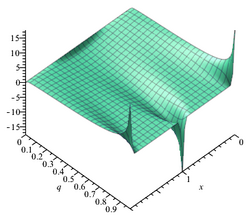
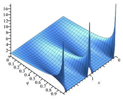


![{\displaystyle {\begin{aligned}\vartheta _{00}\!\left({\frac {z}{\tau }};{\frac {-1}{\tau }}\right)&=\alpha \,\vartheta _{00}(z;\tau )\quad &\vartheta _{01}\!\left({\frac {z}{\tau }};{\frac {-1}{\tau }}\right)&=\alpha \,\vartheta _{10}(z;\tau )\\[3pt]\vartheta _{10}\!\left({\frac {z}{\tau }};{\frac {-1}{\tau }}\right)&=\alpha \,\vartheta _{01}(z;\tau )\quad &\vartheta _{11}\!\left({\frac {z}{\tau }};{\frac {-1}{\tau }}\right)&=-i\alpha \,\vartheta _{11}(z;\tau ).\end{aligned}}}](https://wikimedia.org/api/rest_v1/media/math/render/svg/e38521d263e968c6643113cb856744c3d8417638)
![{\displaystyle {\begin{aligned}\vartheta _{00}(w,q)&=\sum _{n=-\infty }^{\infty }\left(w^{2}\right)^{n}q^{n^{2}}\quad &\vartheta _{01}(w,q)&=\sum _{n=-\infty }^{\infty }(-1)^{n}\left(w^{2}\right)^{n}q^{n^{2}}\\[3pt]\vartheta _{10}(w,q)&=\sum _{n=-\infty }^{\infty }\left(w^{2}\right)^{n+{\frac {1}{2}}}q^{\left(n+{\frac {1}{2}}\right)^{2}}\quad &\vartheta _{11}(w,q)&=i\sum _{n=-\infty }^{\infty }(-1)^{n}\left(w^{2}\right)^{n+{\frac {1}{2}}}q^{\left(n+{\frac {1}{2}}\right)^{2}}.\end{aligned}}}](https://wikimedia.org/api/rest_v1/media/math/render/svg/acbc490b1dd786cc2ef221b6b0834661d3f41ac3)


![{\displaystyle {\begin{aligned}\vartheta _{01}(z\mid q)&=\prod _{m=1}^{\infty }\left(1-q^{2m}\right)\left(1-2\cos(2\pi z)q^{2m-1}+q^{4m-2}\right),\\[3pt]\vartheta _{10}(z\mid q)&=2q^{\frac {1}{4}}\cos(\pi z)\prod _{m=1}^{\infty }\left(1-q^{2m}\right)\left(1+2\cos(2\pi z)q^{2m}+q^{4m}\right),\\[3pt]\vartheta _{11}(z\mid q)&=-2q^{\frac {1}{4}}\sin(\pi z)\prod _{m=1}^{\infty }\left(1-q^{2m}\right)\left(1-2\cos(2\pi z)q^{2m}+q^{4m}\right).\end{aligned}}}](https://wikimedia.org/api/rest_v1/media/math/render/svg/1a2f486ca65bf1df31851e9591220ff601cf6fb0)


![{\displaystyle {\begin{aligned}\vartheta _{00}(z;\tau )&=-i\int _{i-\infty }^{i+\infty }e^{i\pi \tau u^{2}}{\frac {\cos(2\pi uz+\pi u)}{\sin(\pi u)}}\mathrm {d} u;\\[6pt]\vartheta _{01}(z;\tau )&=-i\int _{i-\infty }^{i+\infty }e^{i\pi \tau u^{2}}{\frac {\cos(2\pi uz)}{\sin(\pi u)}}\mathrm {d} u;\\[6pt]\vartheta _{10}(z;\tau )&=-ie^{i\pi z+{\frac {1}{4}}i\pi \tau }\int _{i-\infty }^{i+\infty }e^{i\pi \tau u^{2}}{\frac {\cos(2\pi uz+\pi u+\pi \tau u)}{\sin(\pi u)}}\mathrm {d} u;\\[6pt]\vartheta _{11}(z;\tau )&=e^{i\pi z+{\frac {1}{4}}i\pi \tau }\int _{i-\infty }^{i+\infty }e^{i\pi \tau u^{2}}{\frac {\cos(2\pi uz+\pi \tau u)}{\sin(\pi u)}}\mathrm {d} u.\end{aligned}}}](https://wikimedia.org/api/rest_v1/media/math/render/svg/bd32c29ab16bda39187ec29c1169e8019bcb54af)

![{\displaystyle \theta _{3}(q)=1+{\frac {4q{\sqrt {\ln(1/q)}}}{\sqrt {\pi }}}\int _{0}^{\infty }{\frac {\exp[-\ln(1/q)\,x^{2}]\{1-q^{2}\cos[2\ln(1/q)\,x]\}}{1-2q^{2}\cos[2\ln(1/q)\,x]+q^{4}}}\,\mathrm {d} x}](https://wikimedia.org/api/rest_v1/media/math/render/svg/9e26186736a2e273adfa2732fea7ee65263231d4)
![{\displaystyle {\biggl [}{\frac {2}{\pi }}K{\bigl (}{\frac {1}{2}}{\sqrt {2}}{\bigr )}{\biggr ]}^{1/2}=\theta _{3}{\bigl [}\exp(-\pi ){\bigr ]}=1+4\exp(-\pi )\int _{0}^{\infty }{\frac {\exp(-\pi x^{2})[1-\exp(-2\pi )\cos(2\pi x)]}{1-2\exp(-2\pi )\cos(2\pi x)+\exp(-4\pi )}}\,\mathrm {d} x}](https://wikimedia.org/api/rest_v1/media/math/render/svg/942b823ba5f2a5d89016b6493ca9cc3b187cb86f)
![{\displaystyle {\biggl [}{\frac {2}{\pi }}K({\sqrt {2}}-1){\biggr ]}^{1/2}=\theta _{3}{\bigl [}\exp(-{\sqrt {2}}\,\pi ){\bigr ]}=1+4\,{\sqrt[{4}]{2}}\exp(-{\sqrt {2}}\,\pi )\int _{0}^{\infty }{\frac {\exp(-{\sqrt {2}}\,\pi x^{2})[1-\exp(-2{\sqrt {2}}\,\pi )\cos(2{\sqrt {2}}\,\pi x)]}{1-2\exp(-2{\sqrt {2}}\,\pi )\cos(2{\sqrt {2}}\,\pi x)+\exp(-4{\sqrt {2}}\,\pi )}}\,\mathrm {d} x}](https://wikimedia.org/api/rest_v1/media/math/render/svg/5cc3a6cd1621989208f56af90722f5230eecf7b6)
![{\displaystyle {\biggl \{}{\frac {2}{\pi }}K{\bigl [}\sin {\bigl (}{\frac {\pi }{12}}{\bigr )}{\bigr ]}{\biggr \}}^{1/2}=\theta _{3}{\bigl [}\exp(-{\sqrt {3}}\,\pi ){\bigr ]}=1+4\,{\sqrt[{4}]{3}}\exp(-{\sqrt {3}}\,\pi )\int _{0}^{\infty }{\frac {\exp(-{\sqrt {3}}\,\pi x^{2})[1-\exp(-2{\sqrt {3}}\,\pi )\cos(2{\sqrt {3}}\,\pi x)]}{1-2\exp(-2{\sqrt {3}}\,\pi )\cos(2{\sqrt {3}}\,\pi x)+\exp(-4{\sqrt {3}}\,\pi )}}\,\mathrm {d} x}](https://wikimedia.org/api/rest_v1/media/math/render/svg/9d462b60e5965c30acaf2837ae9770eb3a3560f5)


![{\displaystyle \theta _{3}\left({\frac {1}{2}}\right)=1+2\sum _{n=1}^{\infty }{\frac {1}{2^{n^{2}}}}=1+2\pi ^{-1/2}{\sqrt {\ln(2)}}\int _{0}^{\infty }{\frac {\exp[-\ln(2)\,x^{2}]\{16-4\cos[2\ln(2)\,x]\}}{17-8\cos[2\ln(2)\,x]}}\,\mathrm {d} x}](https://wikimedia.org/api/rest_v1/media/math/render/svg/80285f837f55ecc6e8a2d0b82edd47eb6a50467b)

![{\displaystyle \theta _{3}\left({\frac {1}{3}}\right)=1+2\sum _{n=1}^{\infty }{\frac {1}{3^{n^{2}}}}=1+{\frac {4}{3}}\pi ^{-1/2}{\sqrt {\ln(3)}}\int _{0}^{\infty }{\frac {\exp[-\ln(3)\,x^{2}]\{81-9\cos[2\ln(3)\,x]\}}{82-18\cos[2\ln(3)\,x]}}\,\mathrm {d} x}](https://wikimedia.org/api/rest_v1/media/math/render/svg/b778736b39bddab58af391077803cffab7928c6c)


![{\displaystyle {\begin{aligned}\varphi \left(e^{-\pi }\right)&={\frac {\sqrt[{4}]{\pi }}{\Gamma \left({\frac {3}{4}}\right)}}={\sqrt {2}}\,\eta \left({\sqrt {-1}}\right)\\\varphi \left(e^{-2\pi }\right)&={\frac {\sqrt[{4}]{\pi }}{\Gamma \left({\frac {3}{4}}\right)}}{\frac {\sqrt {2+{\sqrt {2}}}}{2}}\\\varphi \left(e^{-3\pi }\right)&={\frac {\sqrt[{4}]{\pi }}{\Gamma \left({\frac {3}{4}}\right)}}{\frac {\sqrt {1+{\sqrt {3}}}}{\sqrt[{8}]{108}}}\\\varphi \left(e^{-4\pi }\right)&={\frac {\sqrt[{4}]{\pi }}{\Gamma \left({\frac {3}{4}}\right)}}{\frac {2+{\sqrt[{4}]{8}}}{4}}\\\varphi \left(e^{-5\pi }\right)&={\frac {\sqrt[{4}]{\pi }}{\Gamma \left({\frac {3}{4}}\right)}}{\sqrt {\frac {2+{\sqrt {5}}}{5}}}\\\varphi \left(e^{-6\pi }\right)&={\frac {\sqrt[{4}]{\pi }}{\Gamma \left({\frac {3}{4}}\right)}}{\frac {\sqrt {{\sqrt[{4}]{1}}+{\sqrt[{4}]{3}}+{\sqrt[{4}]{4}}+{\sqrt[{4}]{9}}}}{\sqrt[{8}]{12^{3}}}}\\\varphi \left(e^{-7\pi }\right)&={\frac {\sqrt[{4}]{\pi }}{\Gamma \left({\frac {3}{4}}\right)}}{\frac {\sqrt {{\sqrt {13+{\sqrt {7}}}}+{\sqrt {7+3{\sqrt {7}}}}}}{{\sqrt[{8}]{14^{3}}}\cdot {\sqrt[{16}]{7}}}}\\\varphi \left(e^{-8\pi }\right)&={\frac {\sqrt[{4}]{\pi }}{\Gamma \left({\frac {3}{4}}\right)}}{\frac {{\sqrt {2+{\sqrt {2}}}}+{\sqrt[{8}]{128}}}{4}}\\\varphi \left(e^{-9\pi }\right)&={\frac {\sqrt[{4}]{\pi }}{\Gamma \left({\frac {3}{4}}\right)}}{\frac {1+{\sqrt[{3}]{2+2{\sqrt {3}}}}}{3}}\\\varphi \left(e^{-10\pi }\right)&={\frac {\sqrt[{4}]{\pi }}{\Gamma \left({\frac {3}{4}}\right)}}{\frac {\sqrt {{\sqrt[{4}]{64}}+{\sqrt[{4}]{80}}+{\sqrt[{4}]{81}}+{\sqrt[{4}]{100}}}}{\sqrt[{4}]{200}}}\\\varphi \left(e^{-11\pi }\right)&={\frac {\sqrt[{4}]{\pi }}{\Gamma \left({\frac {3}{4}}\right)}}{\frac {\sqrt {11+{\sqrt {11}}+(5+3{\sqrt {3}}+{\sqrt {11}}+{\sqrt {33}}){\sqrt[{3}]{-44+33{\sqrt {3}}}}+(-5+3{\sqrt {3}}-{\sqrt {11}}+{\sqrt {33}}){\sqrt[{3}]{44+33{\sqrt {3}}}}}}{\sqrt[{8}]{52180524}}}\\\varphi \left(e^{-12\pi }\right)&={\frac {\sqrt[{4}]{\pi }}{\Gamma \left({\frac {3}{4}}\right)}}{\frac {\sqrt {{\sqrt[{4}]{1}}+{\sqrt[{4}]{2}}+{\sqrt[{4}]{3}}+{\sqrt[{4}]{4}}+{\sqrt[{4}]{9}}+{\sqrt[{4}]{18}}+{\sqrt[{4}]{24}}}}{2{\sqrt[{8}]{108}}}}\\\varphi \left(e^{-13\pi }\right)&={\frac {\sqrt[{4}]{\pi }}{\Gamma \left({\frac {3}{4}}\right)}}{\frac {\sqrt {13+8{\sqrt {13}}+(11-6{\sqrt {3}}+{\sqrt {13}}){\sqrt[{3}]{143+78{\sqrt {3}}}}+(11+6{\sqrt {3}}+{\sqrt {13}}){\sqrt[{3}]{143-78{\sqrt {3}}}}}}{\sqrt[{4}]{19773}}}\\\varphi \left(e^{-14\pi }\right)&={\frac {\sqrt[{4}]{\pi }}{\Gamma \left({\frac {3}{4}}\right)}}{\frac {\sqrt {{\sqrt {13+{\sqrt {7}}}}+{\sqrt {7+3{\sqrt {7}}}}+{\sqrt {10+2{\sqrt {7}}}}+{\sqrt[{8}]{28}}{\sqrt {4+{\sqrt {7}}}}}}{\sqrt[{16}]{28^{7}}}}\\\varphi \left(e^{-15\pi }\right)&={\frac {\sqrt[{4}]{\pi }}{\Gamma \left({\frac {3}{4}}\right)}}{\frac {\sqrt {7+3{\sqrt {3}}+{\sqrt {5}}+{\sqrt {15}}+{\sqrt[{4}]{60}}+{\sqrt[{4}]{1500}}}}{{\sqrt[{8}]{12^{3}}}\cdot {\sqrt {5}}}}\\2\varphi \left(e^{-16\pi }\right)&=\varphi \left(e^{-4\pi }\right)+{\frac {\sqrt[{4}]{\pi }}{\Gamma \left({\frac {3}{4}}\right)}}{\frac {\sqrt[{4}]{1+{\sqrt {2}}}}{\sqrt[{16}]{128}}}\\\varphi \left(e^{-17\pi }\right)&={\frac {\sqrt[{4}]{\pi }}{\Gamma \left({\frac {3}{4}}\right)}}{\frac {{\sqrt {2}}(1+{\sqrt[{4}]{17}})+{\sqrt[{8}]{17}}{\sqrt {5+{\sqrt {17}}}}}{\sqrt {17+17{\sqrt {17}}}}}\\2\varphi \left(e^{-20\pi }\right)&=\varphi \left(e^{-5\pi }\right)+{\frac {\sqrt[{4}]{\pi }}{\Gamma \left({\frac {3}{4}}\right)}}{\sqrt {\frac {3+2{\sqrt[{4}]{5}}}{5{\sqrt {2}}}}}\\6\varphi \left(e^{-36\pi }\right)&=3\varphi \left(e^{-9\pi }\right)+2\varphi \left(e^{-4\pi }\right)-\varphi \left(e^{-\pi }\right)+{\frac {\sqrt[{4}]{\pi }}{\Gamma \left({\frac {3}{4}}\right)}}{\sqrt[{3}]{{\sqrt[{4}]{2}}+{\sqrt[{4}]{18}}+{\sqrt[{4}]{216}}}}\end{aligned}}}](https://wikimedia.org/api/rest_v1/media/math/render/svg/d06e5700e306ee31cbf5d9565847590b4d4b966a)


![{\displaystyle \varphi {\bigl [}\exp(-{\tfrac {1}{5}}\pi ){\bigr ]}={\sqrt[{4}]{\pi }}\,{\Gamma \left({\tfrac {3}{4}}\right)}^{-1}\operatorname {slh} {\bigl (}{\tfrac {1}{5}}{\sqrt {2}}\,\varpi {\bigr )}\operatorname {slh} {\bigl (}{\tfrac {2}{5}}{\sqrt {2}}\,\varpi {\bigr )}}](https://wikimedia.org/api/rest_v1/media/math/render/svg/087f2996a1cad31a875a6346e7b52be98453668f)
![{\displaystyle \varphi {\bigl [}\exp(-{\tfrac {1}{7}}\pi ){\bigr ]}={\sqrt[{4}]{\pi }}\,{\Gamma \left({\tfrac {3}{4}}\right)}^{-1}\operatorname {slh} {\bigl (}{\tfrac {1}{7}}{\sqrt {2}}\,\varpi {\bigr )}\operatorname {slh} {\bigl (}{\tfrac {2}{7}}{\sqrt {2}}\,\varpi {\bigr )}\operatorname {slh} {\bigl (}{\tfrac {3}{7}}{\sqrt {2}}\,\varpi {\bigr )}}](https://wikimedia.org/api/rest_v1/media/math/render/svg/f01f0cb2fd209abfbb1ac4c204c509f2b3f47b74)
![{\displaystyle \varphi {\bigl [}\exp(-{\tfrac {1}{9}}\pi ){\bigr ]}={\sqrt[{4}]{\pi }}\,{\Gamma \left({\tfrac {3}{4}}\right)}^{-1}\operatorname {slh} {\bigl (}{\tfrac {1}{9}}{\sqrt {2}}\,\varpi {\bigr )}\operatorname {slh} {\bigl (}{\tfrac {2}{9}}{\sqrt {2}}\,\varpi {\bigr )}\operatorname {slh} {\bigl (}{\tfrac {3}{9}}{\sqrt {2}}\,\varpi {\bigr )}\operatorname {slh} {\bigl (}{\tfrac {4}{9}}{\sqrt {2}}\,\varpi {\bigr )}}](https://wikimedia.org/api/rest_v1/media/math/render/svg/51aea624bd4ccfed27077389532d4b07efda771e)
![{\displaystyle \varphi {\bigl [}\exp(-{\tfrac {1}{11}}\pi ){\bigr ]}={\sqrt[{4}]{\pi }}\,{\Gamma \left({\tfrac {3}{4}}\right)}^{-1}\operatorname {slh} {\bigl (}{\tfrac {1}{11}}{\sqrt {2}}\,\varpi {\bigr )}\operatorname {slh} {\bigl (}{\tfrac {2}{11}}{\sqrt {2}}\,\varpi {\bigr )}\operatorname {slh} {\bigl (}{\tfrac {3}{11}}{\sqrt {2}}\,\varpi {\bigr )}\operatorname {slh} {\bigl (}{\tfrac {4}{11}}{\sqrt {2}}\,\varpi {\bigr )}\operatorname {slh} {\bigl (}{\tfrac {5}{11}}{\sqrt {2}}\,\varpi {\bigr )}}](https://wikimedia.org/api/rest_v1/media/math/render/svg/3839f652515fbc383f7fa265b6541beaa7582c59)

![{\displaystyle {\begin{aligned}2\varphi \left(q^{4}\right)&=\varphi (q)+{\sqrt {2\varphi ^{2}\left(q^{2}\right)-\varphi ^{2}(q)}}\\3\varphi \left(q^{9}\right)&=\varphi (q)+{\sqrt[{3}]{9{\frac {\varphi ^{4}\left(q^{3}\right)}{\varphi (q)}}-\varphi ^{3}(q)}}\\{\sqrt {5}}\varphi \left(q^{25}\right)&=\varphi \left(q^{5}\right)\cot \left({\frac {1}{2}}\arctan \left({\frac {2}{\sqrt {5}}}{\frac {\varphi (q)\varphi \left(q^{5}\right)}{\varphi ^{2}(q)-\varphi ^{2}\left(q^{5}\right)}}{\frac {1+s(q)-s^{2}(q)}{s(q)}}\right)\right)\end{aligned}}}](https://wikimedia.org/api/rest_v1/media/math/render/svg/e3a018fbcd1409ba1ebb0c85d8178fb163fa3ba0)

![{\displaystyle {\begin{aligned}s(q)&={\sqrt[{5}]{\tan \left({\frac {1}{2}}\arctan \left({\frac {5}{2}}{\frac {\varphi ^{2}\left(q^{5}\right)}{\varphi ^{2}(q)}}-{\frac {1}{2}}\right)\right)\cot ^{2}\left({\frac {1}{2}}\operatorname {arccot} \left({\frac {5}{2}}{\frac {\varphi ^{2}\left(q^{5}\right)}{\varphi ^{2}(q)}}-{\frac {1}{2}}\right)\right)}}\\&={\cfrac {e^{-\pi i/(25\tau )}}{1-{\cfrac {e^{-\pi i/(5\tau )}}{1+{\cfrac {e^{-2\pi i/(5\tau )}}{1-\ddots }}}}}}\end{aligned}}}](https://wikimedia.org/api/rest_v1/media/math/render/svg/de23ddbf5b96a5a2470d73ba10f05153d2a7e37d)
![{\displaystyle {\begin{array}{lll}\varphi \left(\exp(-{\sqrt {3}}\,\pi )\right)&=&\pi ^{-1}{\Gamma \left({\tfrac {4}{3}}\right)}^{3/2}2^{-2/3}3^{13/8}\\\varphi \left(\exp(-2{\sqrt {3}}\,\pi )\right)&=&\pi ^{-1}{\Gamma \left({\tfrac {4}{3}}\right)}^{3/2}2^{-2/3}3^{13/8}\cos({\tfrac {1}{24}}\pi )\\\varphi \left(\exp(-3{\sqrt {3}}\,\pi )\right)&=&\pi ^{-1}{\Gamma \left({\tfrac {4}{3}}\right)}^{3/2}2^{-2/3}3^{7/8}({\sqrt[{3}]{2}}+1)\\\varphi \left(\exp(-4{\sqrt {3}}\,\pi )\right)&=&\pi ^{-1}{\Gamma \left({\tfrac {4}{3}}\right)}^{3/2}2^{-5/3}3^{13/8}{\Bigl (}1+{\sqrt {\cos({\tfrac {1}{12}}\pi )}}{\Bigr )}\\\varphi \left(\exp(-5{\sqrt {3}}\,\pi )\right)&=&\pi ^{-1}{\Gamma \left({\tfrac {4}{3}}\right)}^{3/2}2^{-2/3}3^{5/8}\sin({\tfrac {1}{5}}\pi )({\tfrac {2}{5}}{\sqrt[{3}]{100}}+{\tfrac {2}{5}}{\sqrt[{3}]{10}}+{\tfrac {3}{5}}{\sqrt {5}}+1)\end{array}}}](https://wikimedia.org/api/rest_v1/media/math/render/svg/913e0c2a4e7f8efd215821d4423789caf3cc7382)
![{\displaystyle {\begin{array}{lll}\varphi \left(\exp(-{\sqrt {2}}\,\pi )\right)&=&\pi ^{-1/2}\Gamma \left({\tfrac {9}{8}}\right){\Gamma \left({\tfrac {5}{4}}\right)}^{-1/2}2^{7/8}\\\varphi \left(\exp(-2{\sqrt {2}}\,\pi )\right)&=&\pi ^{-1/2}\Gamma \left({\tfrac {9}{8}}\right){\Gamma \left({\tfrac {5}{4}}\right)}^{-1/2}2^{1/8}{\Bigl (}1+{\sqrt {{\sqrt {2}}-1}}{\Bigr )}\\\varphi \left(\exp(-3{\sqrt {2}}\,\pi )\right)&=&\pi ^{-1/2}\Gamma \left({\tfrac {9}{8}}\right){\Gamma \left({\tfrac {5}{4}}\right)}^{-1/2}2^{3/8}3^{-1/2}({\sqrt {3}}+1){\sqrt {\tan({\tfrac {5}{24}}\pi )}}\\\varphi \left(\exp(-4{\sqrt {2}}\,\pi )\right)&=&\pi ^{-1/2}\Gamma \left({\tfrac {9}{8}}\right){\Gamma \left({\tfrac {5}{4}}\right)}^{-1/2}2^{-1/8}{\Bigl (}1+{\sqrt[{4}]{2{\sqrt {2}}-2}}{\Bigr )}\\\varphi \left(\exp(-5{\sqrt {2}}\,\pi )\right)&=&\pi ^{-1/2}\Gamma \left({\tfrac {9}{8}}\right){\Gamma \left({\tfrac {5}{4}}\right)}^{-1/2}{\frac {1}{15}}\,2^{3/8}\times \\&&\times {\biggl [}{\sqrt[{3}]{5}}\,{\sqrt {10+2{\sqrt {5}}}}{\biggl (}{\sqrt[{3}]{5+{\sqrt {2}}+3{\sqrt {3}}}}+{\sqrt[{3}]{5+{\sqrt {2}}-3{\sqrt {3}}}}\,{\biggr )}-{\bigl (}2-{\sqrt {2}}\,{\bigr )}{\sqrt {25-10{\sqrt {5}}}}\,{\biggr ]}\\\varphi \left(\exp(-{\sqrt {6}}\,\pi )\right)&=&\pi ^{-1/2}\Gamma \left({\tfrac {5}{24}}\right){\Gamma \left({\tfrac {5}{12}}\right)}^{-1/2}2^{-13/24}3^{-1/8}{\sqrt {\sin({\tfrac {5}{12}}\pi )}}\\\varphi \left(\exp(-{\tfrac {1}{2}}{\sqrt {6}}\,\pi )\right)&=&\pi ^{-1/2}\Gamma \left({\tfrac {5}{24}}\right){\Gamma \left({\tfrac {5}{12}}\right)}^{-1/2}2^{5/24}3^{-1/8}\sin({\tfrac {5}{24}}\pi )\end{array}}}](https://wikimedia.org/api/rest_v1/media/math/render/svg/81f37f7d59609f062b1826b22a23db9ff7a12a95)
![{\displaystyle \theta _{2}(q^{2})={\tfrac {1}{2}}{\sqrt {2[\theta _{3}(q)^{2}-\theta _{4}(q)^{2}]}}}](https://wikimedia.org/api/rest_v1/media/math/render/svg/49fdbf249a5c77891ea7be62a7abdb74bfca9c20)
![{\displaystyle \theta _{3}(q^{2})={\tfrac {1}{2}}{\sqrt {2[\theta _{3}(q)^{2}+\theta _{4}(q)^{2}]}}}](https://wikimedia.org/api/rest_v1/media/math/render/svg/ab78a4868b53c96cb965bc889ba12f8e4fd5bd44)


![{\displaystyle 27\,\theta _{3}(q^{3})^{8}-18\,\theta _{3}(q^{3})^{4}\theta _{3}(q)^{4}-\,\theta _{3}(q)^{8}=8\,\theta _{3}(q^{3})^{2}\theta _{3}(q)^{2}[2\,\theta _{4}(q)^{4}-\theta _{3}(q)^{4}]}](https://wikimedia.org/api/rest_v1/media/math/render/svg/ee8b22b2491acbf41acf156847592744fe5efda4)
![{\displaystyle 27\,\theta _{4}(q^{3})^{8}-18\,\theta _{4}(q^{3})^{4}\theta _{4}(q)^{4}-\,\theta _{4}(q)^{8}=8\,\theta _{4}(q^{3})^{2}\theta _{4}(q)^{2}[2\,\theta _{3}(q)^{4}-\theta _{4}(q)^{4}]}](https://wikimedia.org/api/rest_v1/media/math/render/svg/6db22a825f23c8747194677df1ba5b9cd6776c58)
![{\displaystyle [\theta _{3}(q)^{2}-\theta _{3}(q^{5})^{2}][5\,\theta _{3}(q^{5})^{2}-\theta _{3}(q)^{2}]^{5}=256\,\theta _{3}(q^{5})^{2}\theta _{3}(q)^{2}\theta _{4}(q)^{4}[\theta _{3}(q)^{4}-\theta _{4}(q)^{4}]}](https://wikimedia.org/api/rest_v1/media/math/render/svg/21698abd5cd7e4f2b57023ecd5dd70b3fd545ffb)
![{\displaystyle [\theta _{4}(q^{5})^{2}-\theta _{4}(q)^{2}][5\,\theta _{4}(q^{5})^{2}-\theta _{4}(q)^{2}]^{5}=256\,\theta _{4}(q^{5})^{2}\theta _{4}(q)^{2}\theta _{3}(q)^{4}[\theta _{3}(q)^{4}-\theta _{4}(q)^{4}]}](https://wikimedia.org/api/rest_v1/media/math/render/svg/6bc5563a31bcb890a22ebb282ad224297a82b287)
![{\displaystyle {\biggl [}{\frac {\theta _{3}(q^{1/3})^{2}}{\theta _{3}(q)^{2}}}-{\frac {3\,\theta _{3}(q^{3})^{2}}{\theta _{3}(q)^{2}}}{\biggr ]}^{2}=4-4{\biggl [}{\frac {2\,\theta _{2}(q)^{2}\theta _{4}(q)^{2}}{\theta _{3}(q)^{4}}}{\biggr ]}^{2/3}}](https://wikimedia.org/api/rest_v1/media/math/render/svg/a41eb7bba4644993c0994d693977d751526d68a1)
![{\displaystyle {\biggl [}{\frac {3\,\theta _{4}(q^{3})^{2}}{\theta _{4}(q)^{2}}}-{\frac {\theta _{4}(q^{1/3})^{2}}{\theta _{4}(q)^{2}}}{\biggr ]}^{2}=4+4{\biggl [}{\frac {2\,\theta _{2}(q)^{2}\theta _{3}(q)^{2}}{\theta _{4}(q)^{4}}}{\biggr ]}^{2/3}}](https://wikimedia.org/api/rest_v1/media/math/render/svg/f4d0741127e031b7079dffa001160094eb9b03c9)
![{\displaystyle R(q)=\tan {\biggl \{}{\frac {1}{2}}\arctan {\biggl [}{\frac {1}{2}}-{\frac {\theta _{4}(q)^{2}}{2\,\theta _{4}(q^{5})^{2}}}{\biggr ]}{\biggr \}}^{1/5}\tan {\biggl \{}{\frac {1}{2}}\operatorname {arccot} {\biggl [}{\frac {1}{2}}-{\frac {\theta _{4}(q)^{2}}{2\,\theta _{4}(q^{5})^{2}}}{\biggr ]}{\biggr \}}^{2/5}}](https://wikimedia.org/api/rest_v1/media/math/render/svg/122911c8d5591255a99de086a6643e60e8496af8)
![{\displaystyle R(q^{2})=\tan {\biggl \{}{\frac {1}{2}}\arctan {\biggl [}{\frac {1}{2}}-{\frac {\theta _{4}(q)^{2}}{2\,\theta _{4}(q^{5})^{2}}}{\biggr ]}{\biggr \}}^{2/5}\cot {\biggl \{}{\frac {1}{2}}\operatorname {arccot} {\biggl [}{\frac {1}{2}}-{\frac {\theta _{4}(q)^{2}}{2\,\theta _{4}(q^{5})^{2}}}{\biggr ]}{\biggr \}}^{1/5}}](https://wikimedia.org/api/rest_v1/media/math/render/svg/87bef51d2716d70a8054cd882a9c6a98aa234b16)
![{\displaystyle R(q^{2})=\tan {\biggl \{}{\frac {1}{2}}\arctan {\biggl [}{\frac {\theta _{3}(q)^{2}}{2\,\theta _{3}(q^{5})^{2}}}-{\frac {1}{2}}{\biggr ]}{\biggr \}}^{2/5}\tan {\biggl \{}{\frac {1}{2}}\operatorname {arccot} {\biggl [}{\frac {\theta _{3}(q)^{2}}{2\,\theta _{3}(q^{5})^{2}}}-{\frac {1}{2}}{\biggr ]}{\biggr \}}^{1/5}}](https://wikimedia.org/api/rest_v1/media/math/render/svg/6fd8befdabb6ac82b6c4fff8f0a5bb89a1a5ac55)
![{\displaystyle S(q)={\frac {R(q^{4})}{R(q^{2})R(q)}}=\tan {\biggl \{}{\frac {1}{2}}\arctan {\biggl [}{\frac {\theta _{3}(q)^{2}}{2\,\theta _{3}(q^{5})^{2}}}-{\frac {1}{2}}{\biggr ]}{\biggr \}}^{1/5}\cot {\biggl \{}{\frac {1}{2}}\operatorname {arccot} {\biggl [}{\frac {\theta _{3}(q)^{2}}{2\,\theta _{3}(q^{5})^{2}}}-{\frac {1}{2}}{\biggr ]}{\biggr \}}^{2/5}}](https://wikimedia.org/api/rest_v1/media/math/render/svg/968499610c12ca2700607ba9048ff01e2f8fe303)
![{\displaystyle {\frac {\theta _{3}(q^{1/5})}{\theta _{3}(q^{5})}}-1={\frac {1}{S(q)}}{\bigl [}S(q)^{2}+R(q^{2}){\bigr ]}{\bigl [}1+R(q^{2})S(q){\bigr ]}}](https://wikimedia.org/api/rest_v1/media/math/render/svg/3e1f9826acfe6b0205eb7dec745ce83aae7e6d01)
![{\displaystyle 1-{\frac {\theta _{4}(q^{1/5})}{\theta _{4}(q^{5})}}={\frac {1}{R(q)}}{\bigl [}R(q^{2})+R(q)^{2}{\bigr ]}{\bigl [}1-R(q^{2})R(q){\bigr ]}}](https://wikimedia.org/api/rest_v1/media/math/render/svg/cb6fd08483ead704a199a261edcf54d483835ad9)
![{\displaystyle \theta _{3}(q^{1/5})^{2}-\theta _{3}(q)^{2}={\bigl [}\theta _{3}(q)^{2}-\theta _{3}(q^{5})^{2}{\bigr ]}{\biggl [}1+{\frac {1}{R(q^{2})S(q)}}+R(q^{2})S(q)+{\frac {1}{R(q^{2})^{2}}}+R(q^{2})^{2}+{\frac {1}{S(q)}}-S(q){\biggr ]}}](https://wikimedia.org/api/rest_v1/media/math/render/svg/c87e7c0cdbc5280e1ca49f87d77c2924e364d6c6)
![{\displaystyle \theta _{4}(q)^{2}-\theta _{4}(q^{1/5})^{2}={\bigl [}\theta _{4}(q^{5})^{2}-\theta _{4}(q)^{2}{\bigr ]}{\biggl [}1-{\frac {1}{R(q^{2})R(q)}}-R(q^{2})R(q)+{\frac {1}{R(q^{2})^{2}}}+R(q^{2})^{2}-{\frac {1}{R(q)}}+R(q){\biggr ]}}](https://wikimedia.org/api/rest_v1/media/math/render/svg/6e4601790cf31b8e82943713c410b532e4d75980)
![{\displaystyle \theta _{4}[q(k)]=\theta _{4}[q(k)^{2}]{\sqrt[{8}]{1-k^{2}}}}](https://wikimedia.org/api/rest_v1/media/math/render/svg/ece5e6b2598db08419e115b84fa8dc058e3980b8)
![{\displaystyle \theta _{4}[q(k)^{2}]=\theta _{3}[q(k)]{\sqrt[{8}]{1-k^{2}}}}](https://wikimedia.org/api/rest_v1/media/math/render/svg/85cc179f3c7fab7e4f664ea3a9ad3bed2c751a65)
![{\displaystyle \theta _{3}[q(k)^{2}]=\theta _{3}[q(k)]\cos[{\tfrac {1}{2}}\arcsin(k)]}](https://wikimedia.org/api/rest_v1/media/math/render/svg/9a0b0e95b8b6fd152fc74a01c0f7fbab2b9a6555)
![{\displaystyle \theta _{4}{\biggl \langle }q{\bigl \{}\tan {\bigl [}{\tfrac {1}{2}}\arctan(t^{3}){\bigr ]}{\bigr \}}^{3}{\biggr \rangle }=\theta _{4}{\biggl \langle }q{\bigl \{}\tan {\bigl [}{\tfrac {1}{2}}\arctan(t^{3}){\bigr ]}{\bigr \}}{\biggr \rangle }\,3^{-1/2}{\bigl (}{\sqrt {2{\sqrt {t^{4}-t^{2}+1}}-t^{2}+2}}+{\sqrt {t^{2}+1}}\,{\bigr )}^{1/2}}](https://wikimedia.org/api/rest_v1/media/math/render/svg/0608e409cfd0018afa26a9e4561bc8ce04b7c964)


![{\displaystyle \theta _{4}{\biggl \langle }q{\bigl \{}\tan {\bigl [}{\tfrac {1}{2}}\arctan(1){\bigr ]}{\bigr \}}^{3}{\biggr \rangle }=\theta _{4}{\biggl \langle }q{\bigl \{}\tan {\bigl [}{\tfrac {1}{2}}\arctan(1){\bigr ]}{\bigr \}}{\biggr \rangle }\,3^{-1/2}{\bigl (}{\sqrt {3}}+{\sqrt {2}}\,{\bigr )}^{1/2}}](https://wikimedia.org/api/rest_v1/media/math/render/svg/27d9399dd8871346e454374d0965a18caba1db5c)
![{\displaystyle \theta _{4}{\bigl [}\exp(-3{\sqrt {2}}\,\pi ){\bigr ]}=\theta _{4}{\bigl [}\exp(-{\sqrt {2}}\,\pi ){\bigr ]}\,3^{-1/2}{\bigl (}{\sqrt {3}}+{\sqrt {2}}\,{\bigr )}^{1/2}}](https://wikimedia.org/api/rest_v1/media/math/render/svg/d24c901354972a0b0861ecf1304c11b74666f25b)

![{\displaystyle \theta _{4}{\biggl \langle }q{\bigl \{}\tan {\bigl [}{\tfrac {1}{2}}\arctan(\Phi ^{-6}){\bigr ]}{\bigr \}}^{3}{\biggr \rangle }=\theta _{4}{\biggl \langle }q{\bigl \{}\tan {\bigl [}{\tfrac {1}{2}}\arctan(\Phi ^{-6}){\bigr ]}{\bigr \}}{\biggr \rangle }\,3^{-1/2}{\bigl (}{\sqrt {2{\sqrt {\Phi ^{-8}-\Phi ^{-4}+1}}-\Phi ^{-4}+2}}+{\sqrt {\Phi ^{-4}+1}}\,{\bigr )}^{1/2}}](https://wikimedia.org/api/rest_v1/media/math/render/svg/7dc07d14cd349f46b4f18689ce8fc44277e67902)
![{\displaystyle \theta _{4}{\bigl [}\exp(-3{\sqrt {10}}\,\pi ){\bigr ]}=\theta _{4}{\bigl [}\exp(-{\sqrt {10}}\,\pi ){\bigr ]}\,3^{-1/2}{\bigl (}{\sqrt {2{\sqrt {\Phi ^{-8}-\Phi ^{-4}+1}}-\Phi ^{-4}+2}}+{\sqrt {\Phi ^{-4}+1}}\,{\bigr )}^{1/2}}](https://wikimedia.org/api/rest_v1/media/math/render/svg/76245ff2f6bee7a43882f3f4ebbcad691b406a96)


![{\displaystyle ={\frac {\sqrt {5}}{4}}\,\theta _{2}(\Phi ^{-2})^{2}={\frac {\sqrt {5}}{8}}{\bigl [}\theta _{3}(\Phi ^{-1})^{2}-\theta _{4}(\Phi ^{-1})^{2}{\bigr ]}}](https://wikimedia.org/api/rest_v1/media/math/render/svg/e05e65a1d4c792ec63055ed7d1d9a08f7faf285e)
![{\displaystyle \sum _{n=1}^{\infty }{\frac {1}{F_{2n-1}}}={\frac {\sqrt {5}}{4}}\,{\biggl [}\sum _{n=1}^{\infty }2\,\Phi ^{-(2n-1)^{2}/2}{\biggr ]}^{2}}](https://wikimedia.org/api/rest_v1/media/math/render/svg/e0218550f8623ef9dce9705bde847639ee6e6919)

![{\displaystyle \sum _{n=1}^{\infty }{\frac {1}{F_{n}^{2}}}={\frac {5}{24}}{\bigl [}2\,\theta _{2}(\Phi ^{-2})^{4}-\theta _{3}(\Phi ^{-2})^{4}+1{\bigr ]}={\frac {5}{24}}{\bigl [}\theta _{3}(\Phi ^{-2})^{4}-2\,\theta _{4}(\Phi ^{-2})^{4}+1{\bigr ]}}](https://wikimedia.org/api/rest_v1/media/math/render/svg/71c7f301cb452442a43e1fcd9c91ea78bc820ef9)
![{\displaystyle \sum _{n=1}^{\infty }{\frac {1}{P_{2n-1}}}={\frac {1}{\sqrt {2}}}\,\theta _{2}{\bigl [}({\sqrt {2}}-1)^{2}{\bigr ]}^{2}={\frac {1}{2{\sqrt {2}}}}{\bigl [}\theta _{3}({\sqrt {2}}-1)^{2}-\theta _{4}({\sqrt {2}}-1)^{2}{\bigr ]}}](https://wikimedia.org/api/rest_v1/media/math/render/svg/25a2e2b5ff5d3f65182b77f5be772944bc4d6ea2)
![{\displaystyle {\begin{aligned}\theta _{4}^{2}(q)&=iq^{\frac {1}{4}}\sum _{k=-\infty }^{\infty }q^{2k^{2}-k}\theta _{1}\left({\frac {2k-1}{2i}}\ln q,q\right),\\[6pt]\theta _{4}^{2}(q)&=\sum _{k=-\infty }^{\infty }q^{2k^{2}}\theta _{4}\left({\frac {k\ln q}{i}},q\right).\end{aligned}}}](https://wikimedia.org/api/rest_v1/media/math/render/svg/428f8073ad45e4e54778db88a3dbb2f5b0ab1f30)


![{\displaystyle {\begin{aligned}\vartheta (z;\tau )=\vartheta _{00}(z;\tau )&=0\quad &\Longleftrightarrow &&\quad z&=m+n\tau +{\frac {1}{2}}+{\frac {\tau }{2}}\\[3pt]\vartheta _{11}(z;\tau )&=0\quad &\Longleftrightarrow &&\quad z&=m+n\tau \\[3pt]\vartheta _{10}(z;\tau )&=0\quad &\Longleftrightarrow &&\quad z&=m+n\tau +{\frac {1}{2}}\\[3pt]\vartheta _{01}(z;\tau )&=0\quad &\Longleftrightarrow &&\quad z&=m+n\tau +{\frac {\tau }{2}}\end{aligned}}}](https://wikimedia.org/api/rest_v1/media/math/render/svg/fcdb60358dddb241ffda786440efa91cc0844ca9)


![{\displaystyle {\begin{aligned}\theta _{2}(q)=\vartheta _{10}(0;\tau )&={\frac {2\eta ^{2}(2\tau )}{\eta (\tau )}},\\[3pt]\theta _{3}(q)=\vartheta _{00}(0;\tau )&={\frac {\eta ^{5}(\tau )}{\eta ^{2}\left({\frac {1}{2}}\tau \right)\eta ^{2}(2\tau )}}={\frac {\eta ^{2}\left({\frac {1}{2}}(\tau +1)\right)}{\eta (\tau +1)}},\\[3pt]\theta _{4}(q)=\vartheta _{01}(0;\tau )&={\frac {\eta ^{2}\left({\frac {1}{2}}\tau \right)}{\eta (\tau )}},\end{aligned}}}](https://wikimedia.org/api/rest_v1/media/math/render/svg/2358dd2d333a2740823f158700af932d247a2c7e)


![{\displaystyle E(k)={\frac {\pi }{2}}\sum _{a=0}^{\infty }{\frac {[(2a)!]^{2}}{(1-2a)16^{a}(a!)^{4}}}k^{2a}}](https://wikimedia.org/api/rest_v1/media/math/render/svg/4a4e8c4e1616502c6de3e16bb661c1372b93c0fd)


![{\displaystyle \theta _{2}'(x)={\frac {\mathrm {d} }{\mathrm {d} x}}\,\theta _{2}(x)={\frac {1}{2\pi x}}\theta _{2}(x)\theta _{3}(x)^{2}E{\biggl [}{\frac {\theta _{2}(x)^{2}}{\theta _{3}(x)^{2}}}{\biggr ]}}](https://wikimedia.org/api/rest_v1/media/math/render/svg/0a311084c05bdae1b514737c2f0108933b9f8bae)
![{\displaystyle \theta _{3}'(x)={\frac {\mathrm {d} }{\mathrm {d} x}}\,\theta _{3}(x)=\theta _{3}(x){\bigl [}\theta _{3}(x)^{2}+\theta _{4}(x)^{2}{\bigr ]}{\biggl \{}{\frac {1}{2\pi x}}E{\biggl [}{\frac {\theta _{3}(x)^{2}-\theta _{4}(x)^{2}}{\theta _{3}(x)^{2}+\theta _{4}(x)^{2}}}{\biggr ]}-{\frac {\theta _{4}(x)^{2}}{4\,x}}{\biggr \}}}](https://wikimedia.org/api/rest_v1/media/math/render/svg/104d1b3737a0be4eda8a3a1e245186de9134a6e9)
![{\displaystyle \theta _{4}'(x)={\frac {\mathrm {d} }{\mathrm {d} x}}\,\theta _{4}(x)=\theta _{4}(x){\bigl [}\theta _{3}(x)^{2}+\theta _{4}(x)^{2}{\bigr ]}{\biggl \{}{\frac {1}{2\pi x}}E{\biggl [}{\frac {\theta _{3}(x)^{2}-\theta _{4}(x)^{2}}{\theta _{3}(x)^{2}+\theta _{4}(x)^{2}}}{\biggr ]}-{\frac {\theta _{3}(x)^{2}}{4\,x}}{\biggr \}}}](https://wikimedia.org/api/rest_v1/media/math/render/svg/2f5be9c018c56615a9085df89d3db2ca5d7d26b5)

![{\displaystyle \vartheta _{4}(x){\biggl [}{\frac {\mathrm {d} }{\mathrm {d} x}}\,\vartheta _{3}(x){\biggr ]}-\vartheta _{3}(x){\biggl [}{\frac {\mathrm {d} }{\mathrm {d} x}}\,\theta _{4}(x){\biggr ]}={\frac {1}{4\,x}}\,\theta _{3}(x)\,\theta _{4}(x){\bigl [}\theta _{3}(x)^{4}-\theta _{4}(x)^{4}{\bigr ]}}](https://wikimedia.org/api/rest_v1/media/math/render/svg/b88237a98911175d2efc60c4d21094300a862abd)


![{\displaystyle {\frac {4^{-1/(n+2)}}{n+2}}\csc {\bigl (}{\frac {\pi }{n+2}}{\bigr )}\beta {\biggl [}{\frac {n}{2(n+2)}}{\biggr ]}=\int _{0}^{\infty }{\frac {1}{\sqrt {x^{n+2}+1}}}\,\mathrm {d} x}](https://wikimedia.org/api/rest_v1/media/math/render/svg/48152e52c3eb9c14398e29907e759b53900153c6)
![{\displaystyle {\frac {1}{\sqrt {x^{4}+1}}}={\frac {\mathrm {d} }{\mathrm {d} x}}\,{\frac {1}{2}}F{\biggl [}2\arctan(x);{\frac {1}{2}}{\sqrt {2}}\,{\biggr ]}}](https://wikimedia.org/api/rest_v1/media/math/render/svg/07c42e35cf46076ad7140865bd7327f051d0af90)

![{\displaystyle {\frac {1}{4{\sqrt {2}}}}\csc {\bigl (}{\frac {\pi }{4}}{\bigr )}\beta {\bigl (}{\frac {1}{4}}{\bigr )}=\int _{0}^{\infty }{\frac {1}{\sqrt {x^{4}+1}}}\,\mathrm {d} x={\biggl \{}{\color {blue}{\frac {1}{2}}F{\biggl [}2\arctan(x);{\frac {1}{2}}{\sqrt {2}}\,{\biggr ]}}{\biggr \}}_{x=0}^{x=\infty }=}](https://wikimedia.org/api/rest_v1/media/math/render/svg/ce35084cada7d06712bd0cf775c1560f9a43ab7e)


![{\displaystyle {\frac {1}{\sqrt {x^{6}+1}}}={\frac {\mathrm {d} }{\mathrm {d} x}}\,{\frac {1}{6}}{\sqrt[{4}]{27}}F{\biggl [}2\arctan {\biggl (}{\frac {{\sqrt[{4}]{3}}\,x}{\sqrt {x^{2}+1}}}{\biggr )};{\frac {1}{4}}({\sqrt {6}}+{\sqrt {2}}){\biggr ]}}](https://wikimedia.org/api/rest_v1/media/math/render/svg/3186259fdf61a7ebb632f3d02d679cae524c35f7)

![{\displaystyle {\frac {1}{6{\sqrt[{3}]{2}}}}\csc {\bigl (}{\frac {\pi }{6}}{\bigr )}\beta {\bigl (}{\frac {1}{3}}{\bigr )}=\int _{0}^{\infty }{\frac {1}{\sqrt {x^{6}+1}}}\,\mathrm {d} x={\biggl \{}{\color {blue}{\frac {1}{6}}{\sqrt[{4}]{27}}F{\biggl [}2\arctan {\biggl (}{\frac {{\sqrt[{4}]{3}}\,x}{\sqrt {x^{2}+1}}}{\biggr )};{\frac {1}{4}}({\sqrt {6}}+{\sqrt {2}}){\biggr ]}}{\biggr \}}_{x=0}^{x=\infty }=}](https://wikimedia.org/api/rest_v1/media/math/render/svg/1aeaa28cc9c443e551ccbc434cd63421302cae2b)
![{\displaystyle ={\frac {1}{6}}{\sqrt[{4}]{27}}F{\bigl [}2\arctan({\sqrt[{4}]{3}});{\frac {1}{4}}({\sqrt {6}}+{\sqrt {2}}){\bigr ]}={\frac {2}{9}}{\sqrt[{4}]{27}}K{\bigl [}{\frac {1}{4}}({\sqrt {6}}+{\sqrt {2}}){\bigr ]}={\frac {2}{3}}{\sqrt[{4}]{3}}K{\bigl [}{\frac {1}{4}}({\sqrt {6}}-{\sqrt {2}}){\bigr ]}}](https://wikimedia.org/api/rest_v1/media/math/render/svg/d55b9913617b5871c7a524c0eeec8168828a1c5a)
![{\displaystyle {\color {ForestGreen}K{\bigl [}{\frac {1}{4}}({\sqrt {6}}-{\sqrt {2}}){\bigr ]}={\frac {1}{2{\sqrt[{3}]{2}}{\sqrt[{4}]{3}}}}\beta {\bigl (}{\frac {1}{3}}{\bigr )}}}](https://wikimedia.org/api/rest_v1/media/math/render/svg/fffa258bf7309994a5d54ae0f95d4614975d1ec2)

![{\displaystyle ={\frac {\mathrm {d} }{\mathrm {d} x}}\,{\frac {1}{4}}\sec {\bigl (}{\frac {\pi }{8}}{\bigr )}F{\biggl \{}2\arctan {\biggl [}{\frac {2\cos(\pi /8)\,x}{{\sqrt {x^{4}+{\sqrt {2}}\,x^{2}+1}}-x^{2}+1}}{\biggr ]};2{\sqrt[{4}]{2}}\sin {\bigl (}{\frac {\pi }{8}}{\bigr )}{\biggr \}}+{\frac {1}{4}}\sec {\bigl (}{\frac {\pi }{8}}{\bigr )}F{\biggl \{}\arcsin {\biggl [}{\frac {2\cos(\pi /8)\,x}{x^{2}+1}}{\biggr ]};\tan {\bigl (}{\frac {\pi }{8}}{\bigr )}{\biggr \}}}](https://wikimedia.org/api/rest_v1/media/math/render/svg/9418c896b8d195e1c5bce8b760e71d95bd9cf29e)

![{\displaystyle {\frac {1}{8{\sqrt[{4}]{2}}}}\csc {\bigl (}{\frac {\pi }{8}}{\bigr )}\beta {\bigl (}{\frac {3}{8}}{\bigr )}=\int _{0}^{\infty }{\frac {1}{\sqrt {x^{8}+1}}}\,\mathrm {d} x=}](https://wikimedia.org/api/rest_v1/media/math/render/svg/21e13acda89a6825a0a7a6477bf0e2d072b3ce9e)
![{\displaystyle ={\biggl \langle }{\color {blue}{\frac {1}{4}}\sec {\bigl (}{\frac {\pi }{8}}{\bigr )}F{\biggl \{}2\arctan {\biggl [}{\frac {2\cos(\pi /8)\,x}{{\sqrt {x^{4}+{\sqrt {2}}\,x^{2}+1}}-x^{2}+1}}{\biggr ]};2{\sqrt[{4}]{2}}\sin {\bigl (}{\frac {\pi }{8}}{\bigr )}{\biggr \}}+{\frac {1}{4}}\sec {\bigl (}{\frac {\pi }{8}}{\bigr )}F{\biggl \{}\arcsin {\biggl [}{\frac {2\cos(\pi /8)\,x}{x^{2}+1}}{\biggr ]};\tan {\bigl (}{\frac {\pi }{8}}{\bigr )}{\biggr \}}}{\biggr \rangle }_{x=0}^{x=\infty }=}](https://wikimedia.org/api/rest_v1/media/math/render/svg/5ab622f4004af8bce9bb3de38a20ecb4d4219a21)
![{\displaystyle ={\frac {1}{4}}\sec {\bigl (}{\frac {\pi }{8}}{\bigr )}F{\bigl [}\pi ;2{\sqrt[{4}]{2}}\sin {\bigl (}{\frac {\pi }{8}}{\bigr )}{\bigr ]}={\frac {1}{2}}\sec {\bigl (}{\frac {\pi }{8}}{\bigr )}K({\sqrt {2{\sqrt {2}}-2}}{\bigr )}=2\sin {\bigl (}{\frac {\pi }{8}}{\bigr )}K({\sqrt {2}}-1)}](https://wikimedia.org/api/rest_v1/media/math/render/svg/85a8ad3dc4c269cf0392b1260587f5471ae5e932)
![{\displaystyle {\color {ForestGreen}K({\sqrt {2}}-1)={\frac {1}{8}}{\sqrt[{4}]{2}}\,({\sqrt {2}}+1)\,\beta {\bigl (}{\frac {3}{8}}{\bigr )}}}](https://wikimedia.org/api/rest_v1/media/math/render/svg/177a0e98ca0233f21a20d37c9dd285369ecf1cda)

![{\displaystyle q[{\tfrac {1}{4}}({\sqrt {6}}-{\sqrt {2}})]=\exp(-{\sqrt {3}}\,\pi )}](https://wikimedia.org/api/rest_v1/media/math/render/svg/93d8a66693d1cd78fa0422519e6a5f523cfa1f69)

![{\displaystyle \theta _{3}[q(k)]={\sqrt {2\pi ^{-1}K(k)}}}](https://wikimedia.org/api/rest_v1/media/math/render/svg/f5de1ea9f13775acb606c8cb4c2c8268c77ad546)
![{\displaystyle \theta _{3}[\exp(-\pi )]=\theta _{3}[q({\tfrac {1}{2}}{\sqrt {2}})]={\sqrt {2\pi ^{-1}K({\tfrac {1}{2}}{\sqrt {2}})}}=2^{-1/2}\pi ^{-1/2}\beta ({\tfrac {1}{4}})^{1/2}=2^{-1/4}{\sqrt[{4}]{\pi }}\,{\Gamma {\bigl (}{\tfrac {3}{4}}{\bigr )}}^{-1}}](https://wikimedia.org/api/rest_v1/media/math/render/svg/0c3b3090803e98069d65099cffee88f085fb58b6)
![{\displaystyle \theta _{3}[\exp(-{\sqrt {3}}\,\pi )]=\theta _{3}{\bigl \{}q{\bigl [}{\tfrac {1}{4}}({\sqrt {6}}-{\sqrt {2}}){\bigr ]}{\bigr \}}={\sqrt {2\pi ^{-1}K{\bigl [}{\tfrac {1}{4}}({\sqrt {6}}-{\sqrt {2}}){\bigr ]}}}=2^{-1/6}3^{-1/8}\pi ^{-1/2}\beta ({\tfrac {1}{3}})^{1/2}}](https://wikimedia.org/api/rest_v1/media/math/render/svg/2456d11eb2e069e9d2eac7d2cc91561418429672)
![{\displaystyle \theta _{3}[\exp(-{\sqrt {2}}\,\pi )]=\theta _{3}[q({\sqrt {2}}-1)]={\sqrt {2\pi ^{-1}K({\sqrt {2}}-1)}}=2^{-1/8}\cos({\tfrac {1}{8}}\pi )\,\pi ^{-1/2}\beta ({\tfrac {3}{8}})^{1/2}}](https://wikimedia.org/api/rest_v1/media/math/render/svg/81e6d7302b7c5a86bd706212afbf5c0dddc4be6d)
![{\displaystyle \theta _{4}[q(k)]={\sqrt[{4}]{1-k^{2}}}\,{\sqrt {2\pi ^{-1}K(k)}}}](https://wikimedia.org/api/rest_v1/media/math/render/svg/b18cb501a0e5521687946e420015ea2bfb8e9367)
![{\displaystyle \theta _{4}[\exp(-{\sqrt {2}}\,\pi )]=\theta _{4}[q({\sqrt {2}}-1)]={\sqrt[{4}]{2{\sqrt {2}}-2}}\,{\sqrt {2\pi ^{-1}K({\sqrt {2}}-1)}}=2^{-1/4}\cos({\tfrac {1}{8}}\pi )^{1/2}\,\pi ^{-1/2}\beta ({\tfrac {3}{8}})^{1/2}}](https://wikimedia.org/api/rest_v1/media/math/render/svg/07c0cdf2fb31e0ad42c1c55d8562d70da28f2203)


![{\displaystyle \sum _{k=0}^{\infty }P(k)x^{k}={\frac {1}{(x;x)_{\infty }}}=\theta _{3}(x)^{-1/6}\theta _{4}(x)^{-2/3}{\biggl [}{\frac {\theta _{3}(x)^{4}-\theta _{4}(x)^{4}}{16\,x}}{\biggr ]}^{-1/24}}](https://wikimedia.org/api/rest_v1/media/math/render/svg/d45936d0522b1f639420fa97f49e237424fa4a51)
![{\displaystyle (x;x)_{\infty }=1+\sum _{n=1}^{\infty }{\bigl [}-x^{{\text{Fn}}(2n-1)}-x^{{\text{Kr}}(2n-1)}+x^{{\text{Fn}}(2n)}+x^{{\text{Kr}}(2n)}{\bigr ]}}](https://wikimedia.org/api/rest_v1/media/math/render/svg/eab59cb2fcf2f3ddc6f1e10561a526de51f516f3)


![{\displaystyle \sum _{k=0}^{\infty }Q(k)x^{k}={\frac {1}{(x;x^{2})_{\infty }}}=\theta _{3}(x)^{1/6}\theta _{4}(x)^{-1/3}{\biggl [}{\frac {\theta _{3}(x)^{4}-\theta _{4}(x)^{4}}{16\,x}}{\biggr ]}^{1/24}}](https://wikimedia.org/api/rest_v1/media/math/render/svg/faf3d08f52a11ebbc9e5b9289d4f784f60f103d7)


![{\displaystyle \theta _{4}(x)={\biggl [}\sum _{k=0}^{\infty }P(k)x^{k}{\biggr ]}^{-1}{\biggl [}\sum _{k=0}^{\infty }Q(k)x^{k}{\biggr ]}^{-1}}](https://wikimedia.org/api/rest_v1/media/math/render/svg/4ed01dd893d339d67b7cffd351479d11bd83f819)


